2.3 Measures of Location

The measures of location or position are associated with location parameters.

2.3.1 Minimum and Maximum

The minimum of a distribution is the smallest observed value of that distribution; analogously, the maximum is the largest value. They are order statistics, more specifically the extremes of a(n ordered) list. For a distribution of \(n\) elements they are denoted by \(\min X = x_{(1)}\) and \(\max X = x_{(n)}\).

Despite the simplicity of these measures, there are sophisticated theoretical considerations about them. For more details, see (S. Kotz and Nadarajah 2000).

Example 2.35 (Minimum and maximum) Assume again the \(n=100\) observations of the variable Y: ‘height of women assisted in a hospital’, presented in Example 2.25. The minimum and maximum are denoted, respectively, by \(\min Y = y_{(1)} = 1.51\) and \(\max Y = y_{(100)} = 1.74\).

h <- read.csv('https://filipezabala.com/data/hospital.csv')
min(h$height)     # Minimum

## [1] 1.51

max(h$height)     # Maximum

## [1] 1.74

range(h$height)   # The function 'range' gives the minimum and maximum

## [1] 1.51 1.74

Example 2.36 In Python.

import pandas as pd

# Load the dataset
h = pd.read_csv('https://filipezabala.com/data/hospital.csv')

# Minimum
print(min(h['height'])) # Output: 1.47

# Maximum
print(max(h['height'])) # Output: 1.83

# The np.ptp() function provides the minimum and maximum
print(np.ptp(h['height'])) # Output: 0.36

2.3.2 Total

Total or summation (see Section 1.8) is the sum of all values of a variable. It is expressed by the equations (2.11) and (2.12).

\[\begin{equation} \tau = \sum_{i=1}^N x_i \tag{2.11} \end{equation}\]

\[\begin{equation} \hat{\tau} = N \bar{x}_{n}, \tag{2.12} \end{equation}\]

where \(\bar{x}_{n}\) is the sample mean, presented in Equation (2.14).

Example 2.37 (Total) Reassume the data from Example 2.39. If someone needs a trash can 60 times in the capital of Rio Grande do Sul, it is estimated that the total number of steps to be walked is \[\hat{\tau} = \frac{60}{6} \times 930 = 60 \times 155 = 9300\]

N <- 60                         # Universe/population size
x <- c(186,402,191,20,7,124)    # Raw data
N*mean(x)                       # Equation (2.11)

## [1] 9300

Example 2.38 In Python.

import numpy as np

# Universe/Population Size
N = 60

# Raw Data
x = np.array([186, 402, 191, 20, 7, 124])

# Equation (2.11)
total = N * np.mean(x)
print(total) # Output: 18900.0

2.3.3 (Arithmetic) Mean

The (arithmetic) mean or (arithmetic) average is one of the most important measures in Statistics due to its properties and relative ease of calculation. The mean of the variable \(X\) is generically symbolized by \(\mu\) when referring to the universal mean, and by \(\bar{x}\) when referring to the sample mean. You can use the notation \(\bar{x}_{n}\) to indicate the sample size. Their expressions in universe and in the sample are respectively given by the equations (2.13) and (2.14). Because it distributes the sum of the distribution values over the number of observations, the mean is a measure that indicates the center of mass. \[\begin{equation} \mu = \frac{\sum_{i=1}^N x_i}{N} \tag{2.13} \end{equation}\]

\[\begin{equation} \bar{x}_{n} = \frac{\sum_{i=1}^n x_i}{n} \tag{2.14} \end{equation}\]

Example 2.39 (Arithmetic mean) Assume again the data from Example 1.13. The average number of steps to the nearest trash can was \[\bar{x}_6 = \frac{\sum_{i=1}^6 x_i}{6} = \frac{186+402+191+20+7+124}{6} = \frac{930}{6} = 155.\]

x <- c(186,402,191,20,7,124)      # Raw data
mean(x)                           # Equations (2.8) and (2.9). See ?mean

## [1] 155

Example 2.40 In Python.

import numpy as np

# Raw data
x = np.array([186, 402, 191, 20, 7, 124])

# Calculating the mean
mean = np.mean(x)
print(media) # Output: 155.0

2.3.3.1 Law of Large Numbers

The law of large numbers (LLN) was proposed by (Poisson 1837, 7), and “[c]onsists in the fact that, if we observe a considerable number of events of the same nature, (…) we will find, among these numbers, approximately constant relations”¹¹. Nowadays, we speak of the laws of large numbers, since there are different results involving the original proposal. Essentially, the LGN states that the sample mean \(\bar{x}_n\) converges to the universal mean \(\mu\) when \(n \rightarrow \infty\). (Samuel Kotz et al. 2005, 3979) define three variants, of which the two best known are listed. For details of Erdös-Rényi’s law of large numbers, see (Erdös and Rényi 1970).

Borel’s (strong) law of large numbers If \(X_1,\ldots,X_n\) is a sequence of conditionally independent, identically distributed random variables \(\mathcal{Ber}(\theta)\), i.e., \(Pr(X_i = 1)=\theta\) and \(Pr(X_i = 0)=1-\theta\) for all \(i = 1,\ldots,n\), then \(\bar{x}_n \rightarrow \theta\) almost certainly when \(n \rightarrow \infty\), i.e., \[\begin{equation} Pr\left[ \lim_{n \rightarrow \infty} \frac{\sum_{i=1}^n X_i}{n} = \theta \right] = 1 \tag{2.15} \end{equation}\]

Chebyshev’s (weak) law of large numbers If \(X_1,\ldots,X_n\) is a sequence of conditionally independent random variables such as \(E(X_i)=m_i\) and \(Var(X_i)=\sigma_i^2\), \(i = 1,\ldots,n\), and \(\sigma_i^2 \le c < \infty\), then for any \(\varepsilon > 0\), \(\bar{x}_n \rightarrow \mu\) in probability when \(n \rightarrow \infty\), i.e., \[\begin{equation} \lim_{n \rightarrow \infty} Pr\left[ \left| \frac{\sum_{i=1}^n X_i}{n} - \frac{\sum_{i=1}^n m_i}{n} \right| < \varepsilon \right] = 1 \tag{2.16} \end{equation}\]

Example 2.41 Suppose \(M=20,000\) rolls of a balanced die. From Eq. (3.44) we know that the expected value in this case is \(E(X)=\frac{1+2+3+4+5+6}{6}=3.5\).

M <- 20000
theta <- 1/6
media <- vector(length = M)
sim <- base::sample(1:6, M, replace = TRUE, prob = rep(theta,6))
for(i in 1:M){
  set.seed(i+314); media[i] <- mean(sim[1:i])
}
plot(media, type = 'l', las = 1,
     main = '20,000 rolls of a balanced die')
EX <- mean(1:6)
abline(h = EX, col = 'red')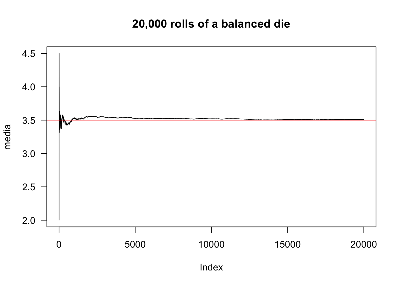

Example 2.42 In Python.

import numpy as np
import matplotlib.pyplot as plt

# Parameters
M = 20000
theta = 1/6

# Simulation
average = np.zeros(M)
yes = np.random.choice(np.arange(1, 7), size=M, 
                       replace=True, p=np.repeat(theta, 6))

for i in range(1, M + 1): 
  np.random.seed(i + 314) 
mean[i - 1] = np.mean(sim[:i])

# Plot
plt.plot(media, linestyle='-', color='blue')
plt.xlabel('Number of releases')
plt.ylabel('Average accumulated')
plt.title('20,000 rolls of a balanced die')

# Expected value
EX = np.mean(np.arange(1, 7))
plt.axhline(y=EX, color='red', linestyle='--')

plt.show()

Exercise 2.8 Consider Example 2.41.
a. Implement for two dice.
b. Vary the number of simulations \(M\).

2.3.3.2 Weighted (arithmetic) mean

The weighted (arithmetic) mean allows to assign different weights to observations.

\[\begin{equation} \bar{x}_{n} = \frac{\sum_{i=1}^n w_i x_i}{\sum_{i=1}^n w_i} \tag{2.17} \end{equation}\]

Example 2.43 (Mate water) Weighted average is like adding hot and cold water to regulate the temperature of the mate. Suppose 1 liter of water in a thermos, where \(w_1=850\)mL (85%) of water is placed at \(x_1=96\,^{\circ}{\rm C}\) and \(w_2=150\)mL (15%) of water at \(x_2=30\,^{\circ}{\rm C}\). Disregarding external variations, this mixture should be \[ W = \frac {850mL \times 96\,^{\circ}{\rm C} + 150mL \times 30\,^{\circ}{\rm C}}{850mL + 150mL} = 0.85 \times 96\,^{\circ}{\rm C}+0.15 \times 30\,^{\circ}{\rm C} = 86.1\,^{\circ}{\rm C}.\]

weighted.mean(c(96,30), c(850,150)) # Makes it a lot easier

## [1] 86.1

Example 2.44 In Python.

import numpy as np

# Data
values = np.array([96, 30])
weights = np.array([850, 150])

# Weighted average
weighted_average = np.average(values, weights=weights)
print(weighted_average) # Output: 85.2

2.3.3.3 Trimmed Mean

Trimming an array of data means trimming a fraction (usually between 0 and 0.5) from each end of the sorted array. The trimmed mean consists of calculating the simple arithmetic mean of the trimmed vector. A formal definition can be found at (Yuen 1974, 166).

x <- c(2:99,1000,10000) # Original vector, containing extreme values
mean(x)                 # Arithmetic mean

## [1] 159.49

mean(x, trim = 0.01)    # Removes 1% of extreme values

## [1] 60.68367347

mean(sort(x[2:99]))     # mean(x, trim = 0.01)

## [1] 60.68367347

mean(x, trim = 0.25)    # Interquartile mean: removes 25% of extreme values

## [1] 51.5

mean(sort(x[26:75]))    # mean(x, trim = 0.25)

## [1] 51.5

Example 2.45 In Python.

import numpy as np

# Original vector, containing extreme values
x = np.array(list(range(2, 100)) + [1000, 10000])

# Arithmetic mean
print(np.mean(x)) # Output: 154.5

# Removes 1% of extreme values
print(np.mean(x, trim=0.01)) # Output: 50,495

# Equivalent to mean(x, trim = 0.01)
x_sorted = np.sort(x)
n = len(x)
trim_index = int(0.01 * n)
print(np.mean(x_sorted[trim_index:n - trim_index])) # Output: 50,495

# Mean interquartile: removes 25% of extreme values
print(np.mean(x, trim=0.25)) # Output: 50.5

# Equivalent to mean(x, trim = 0.25)
x_sorted = np.sort(x)
n = len(x)
trim_index = int(0.25 * n)
print(np.mean(x_sorted[trim_index:n - trim_index])) # Output: 50.5

2.3.3.4 Winsorized Mean

Winsorize an (ordered) array means replacing a certain proportion of extreme values with less extreme values. Thus, the surrogate values are the most extreme retained values. A formal definition can be found at (Yuen 1974, 166).

x <- c(2:99,1000,10000) # Original vector, containing extreme values
xw <- DescTools::Winsorize(x, val=quantile(x, probs=c(0.01, 0.99)))
mean(x)

## [1] 159.49

mean(xw)

## [1] 70.3999

Example 2.46 In Python.

import numpy as np
from scipy.stats.mstats import winsorize

# Original vector, containing extreme values
x = np.array(list(range(2, 100)) + [1000, 10000])

# Calculating quantiles for winsorization
lower_limit = np.quantile(x, 0.01)
upper_limit = np.quantile(x, 0.99)

# Applying winsorization
xw = winsorize(x, limits=(0.01, 0.01))

# Original mean
print(np.mean(x)) # Output: 154.5

# Winsorized mean
print(np.mean(xw)) # Output: 50.99

2.3.4 Mean Square

The mean square is the mean of the squared values, used in the calculation of variances. It is also known as the second moment (not centered). \[\begin{equation} MS = \frac{\sum_{i=1}^n x_{i}^{2}}{n}. \tag{2.18} \end{equation}\]

The root mean square (RMS) is the square root of the mean square. \[\begin{equation} RMS=\sqrt{MS}. \tag{2.19} \end{equation}\]

Example 2.47 (MS and RMS) The mean square of the values 186, 402, 191, 20, 7 and 124 is \[MS = \frac{\sum_{i=1}^6 x_{i}^{2}}{6} = \frac{186^2+402^2+191^2+20^2+7^2+124^2}{6} = \frac{248506}{6} = 41417.\bar{6}.\] The RMS (root mean square) is \[RMS = \sqrt{41417.\bar{6}} \approx 203.5133.\]

x <- c(186,402,191,20,7,124)    # Raw data
(ms <- mean(x^2))               # Eq. (2.12), compare with mean(x)^2

## [1] 41417.66667

sqrt(ms)                        # Eq. (2.13), RMS (root mean square)

## [1] 203.5133083

Example 2.48 In Python.

import numpy as np

# Raw data
x = np.array([186, 402, 191, 20, 7, 124])

# Eq. (2.12)
ms = np.mean(x**2)
print(ms) # Output: 36928.333333333336

# Comparing with mean(x)^2
print(np.mean(x)**2) # Output: 24025.0

# Eq. (2.13)
rms = np.sqrt(ms)
print(rms) # Output: 192.16745259789917

2.3.5 Harmonic Mean

The harmonic mean is used to calculate average rates. It is defined by \[\begin{equation} H = \frac{n}{\frac{1}{x_1} + \frac{1}{x_2} + \cdots + \frac{1}{x_n}} = \frac{n}{\sum_{i=1}^n \frac{1}{x_i}}. \tag{2.20} \end{equation}\]

Example 2.49 (Harmonic mean) Suppose a vehicle traveled a certain distance at 60 km/h and the same distance again at 90 km/h. Its average speed can be calculated by the harmonic mean \[H = \frac{2}{\frac{1}{60} + \frac{1}{90}} = 72 km/h,\] i.e., if the vehicle traveled the entire distance at 72 km/h, it would complete the journey in the same time.

2/((1/60)+(1/90))  # By Equation (2.20)

## [1] 72

1/mean(1/c(60,90)) # Alternative

## [1] 72

Example 2.50 In Python.

import numpy as np

# By Equation (2.20)
result1 = 2 / ((1/60) + (1/90))
print(result1) # Output: 72.0

# Alternative
result2 = 1 / np.mean(1 / np.array([60, 90]))
print(result2) # Output: 72.0

2.3.6 Geometric Mean

The geometric mean is one of the three Pythagorean means, used to represent sets that behave as a geometric progression.¹² Raul Rodrigues de Oliveira at Brasil Escola UOL

The geometric mean is used to calculate averages of indices and accelerations, as well as in cases where the measurements have different numerical magnitudes. It is defined by \[\begin{equation} G = \sqrt[n]{\Pi_{i=1}^n x_i}. \tag{2.21} \end{equation}\]

Example 2.51 (Geometric mean) Let the price indices be \(L_{2004,2008}^{P} = 139.58\%\) and \(P_{2004,2008}^{P} = 97.22\%.\) Its geometric mean is known as Fisher’s (ideal) index, given by \[G = \sqrt{1.3958 \times 0.9722} \approx 116.49\%.\]

sqrt(1.3958*.9722)

## [1] 1.164902039

Example 2.52 In Python.

import math

# Calculating the square root
result = math.sqrt(1.3958 * 0.9722)
print(result) # Output: 1.1650062234417873

2.3.7 Relationship between means

Let \(H\) be the harmonic mean (Eq. (2.20)), \(G\) be the geometric mean (Eq. (2.21)), \(A \equiv \mu\) be the arithmetic mean (Eq. (2.13)), and \(Q \equiv MS\) be the quadratic mean (Eq. (2.18)). If applied to positive values, then \[H \le G \le A \le Q.\]

2.3.8 Mode

Mode(s) is (are) the most frequent value(s) in a distribution. When data are grouped, the modal class must be indicated, i.e., the class with the highest frequency. The computational effort to calculate the mode is to perform a count.

• Amodal: no mode
• Unimodal: one mode
• Bimodal: two modes
• Trimodal: three modes
• Polymodal: four or more modes

In R there is functions like pracma::Mode, but it only works well in the unimodal case. Therefore, the Modes function is presented below, adapted from the suggestion by digEmAll in this StackOverflow discussion. The following examples compare the two approaches.

# Modes function
Modes <- function(x){
  ux <- sort(unique(x))
  tab <- tabulate(match(x, ux))
  if(sum(diff(tab)^2) == 0){
    return('Amodal')
  } else{
    return(ux[tab == max(tab)]) 
  }
}

Example 2.53 In Python.

import numpy as np
from scipy import stats

def Modes(x):
"""
Calculates the mode (or modes) of a dataset.

Args:
x: A NumPy array or list of values.

Returns:
A NumPy array containing the mode(s) of the dataset.
If all values have the same frequency, returns None.
"""
ux = np.sort(np.unique(x))
tab = np.bincount(np.searchsorted(ux, x))
# Check if all values have the same frequency
if np.all(tab == tab[0]):
return None
else:
return ux[tab == np.max(tab)]

Example 2.54 (Unimodal) The mode of the data set 4, 7, 1, 3, 3, 9 is \(Mo=3\), as it has a frequency of 2 while the other values have a frequency of 1. This is a unimodal distribution.

dat <- c(4,7,1,3,3,9)
Modes(dat)

## [1] 3

pracma::Mode(dat)

## [1] 3

Example 2.55 In Python.

import numpy as np
from scipy import stats

dat = np.array([4, 7, 1, 3, 3, 9])

# Using the Modes() function
print(Modes(dat)) # Output: [3]

# Using scipy.stats.mode() (similar to pracma::Mode(dat))
moda, contagem = stats.mode(dat)
print(moda) # Output: [3]

Example 2.56 (Bimodal) The modes of the data set 4, 7, 1, 3, 3, 9, 7 are \(Mo'=3\) and \(Mo''=7\), as both have frequency 2 while the other values have frequency 1. The order of presentation is indifferent. This is a bimodal distribution.

dat <- c(4,7,1,3,3,9,7)
Modes(dat)

## [1] 3 7

pracma::Mode(dat)

## [1] 3

Example 2.57 (Amodal) The data set 4, 7, 1, 3, 9 is said to be amodal because all values have frequency 1.

dat <- c(4,7,1,3,9)
Modes(dat)    # If every value is mode, any value is mode

## [1] "Amodal"

pracma::Mode(dat)

## [1] 1

Example 2.58 In Python.

import numpy as np
from scipy import stats

dat = np.array([4, 7, 1, 3, 9])

# Using the Modes() function
print(Modes(dat)) # Output: None

# Using scipy.stats.mode() (similar to pracma::Mode(dat))
moda, contagem = stats.mode(dat)
print(moda) # Output: [1]

Example 2.59 (Mode for grouped data) In the Example 2.25 it is observed that \(f_{3}=41\) is the highest frequency. The modal class is therefore the third, comprised between the values 1.60 and 1.65.

2.3.9 Quantile

Quantiles or separatrices are measures that divide an ordered set of data into \(k\) equal parts. The basic method consists of obtaining a roll of data and finding (albeit approximately) the values that divide the distribution according to the desired \(k\). The computational effort to calculate any separatrix is, therefore, the sorting of the data. In general, a separatrix \(S\) can be defined according to Eq. (2.22), where \(n\) indicates the number of observations and \(p\) the proportion of observations ordered below \(S\). \[\begin{equation} S = x_{(p(n+1))} \tag{2.22} \end{equation}\]

The stats::quantile() function has nine methods for obtaining quatiles, so the documentation is recommended for more details. With it, you can easily obtain the desired quantiles, just by adjusting the \(p\) argument. Note that the function returns the quantiles expressed in percentiles, where \(0\%\) equals the minimum and \(100\%\) the maximum.

2.3.9.1 Median

The median is the measure that divides half of the ordered data to its left and the other half to its right. It may be described as the \(\frac{1+n}{2}\)th order statistics according to Eq. (2.24). It is the central measure in terms of ordering, and its position is the average between the first and last positions according to Eq. (2.23). \[\begin{equation} Pos = \frac{1+n}{2} \tag{2.23} \end{equation}\]

\[\begin{equation} Md = x_{\left( \frac{1+n}{2} \right)} \tag{2.24} \end{equation}\]

Example 2.60 (Median for odd \(n\)) Consider the regular sequence from \(0\) to \(100\). The position of the median is \(Pos = \frac{1+101}{2}=51\), therefore \(Md=x_{(51)}=50\).

x <- 0:100
sort(x)[51]

## [1] 50

median(x)

## [1] 50

quantile(x, 1/2)

## 50% 
##  50

Example 2.61 In Python.

import numpy as np

x = np.arange(0, 101)

# Sorting x and getting the 51st element
print(np.sort(x)[50]) # Output: 50

# Calculating the median
print(np.median(x)) # Output: 50.0

# Calculating the 1/2 quantile (equivalent to the median)
print(np.quantile(x, 1/2)) # Output: 50.0

Example 2.62 (Median for \(n\) even) When the number of observations is even, just take the average of the two central values of the roll. Let the data set be \(15, -4, 11, 12, 1, 5\), formed by \(n=6\) values. When ordered, we obtain the list \(-4, 1, 5, 11, 12, 15\). Considering again \(k=2\), we obtain the quantile \(Md=\frac{5+11}{2}=8\), because it divides the set into two parts of the same size (three values below 8 and three values above). Its position is given by \(Pos=\frac{1+6}{2}=3.5\), i.e., the median is an intermediate value between the third and fourth positions.

x <- c(15, -4, 11, 12, 1, 5)
(n <- length(x))

## [1] 6

(pos <- (n+1)/2)

## [1] 3.5

sort(x)

## [1] -4  1  5 11 12 15

median(x)

## [1] 8

Example 2.63 In Python.

import numpy as np

x = np.array([15, -4, 11, 12, 1, 5])

# Calculating the size of the array
n = len(x)
print(n) # Output: 6

# Calculating the position of the median
pos = (1 + n) / 2
print(pos) # Output: 3.5

# Sorting the array
x_sorted = np.sort(x)
print(x_sorted) # Output: [-4 1 5 11 12 15]

# Calculating the median
print(np.median(x)) # Output: 8.0

2.3.9.2 Quartiles

The positions of the first and third quartiles can be defined respectively by Eq. (2.25) and (2.26). This is the \(\hat{Q}_6(p)\) algorithm as per (Hyndman and Fan 1996), or type=6 in the stats::quantile() function.

\[\begin{equation} Pos_{\frac{1}{4}} = \frac{1+n}{4} \tag{2.25} \end{equation}\]

\[\begin{equation} Pos_{\frac{3}{4}} = \frac{3(1+n)}{4} \tag{2.26} \end{equation}\]

The first and third quartiles can be defined respectively by Eq. (2.27) and (2.28).

\[\begin{equation} Q_1 = x_{\left( \frac{1+n}{4} \right)} \tag{2.27} \end{equation}\]

\[\begin{equation} Q_3 = x_{\left( \frac{3(1+n)}{4} \right)} \tag{2.28} \end{equation}\]

Example 2.64 Consider again the regular sequence from 0 to 100. The position of the first quartile is \(Pos_{\frac{1}{4}} = \frac{1+101}{4}=25.5\), and that of the third quartile is \(Pos_{\frac{3}{4}} = \frac{3(1+101)}{4}=76.5\). Therefore \(Q_1=x_{(25.5)}=\frac{x_{(25)}+x_{(26)}}{2}=\frac{24+25}{2}=24.5\) and \(Q_3=x_{(76.5)}=\frac{x_{(76)}+x_{(77)}}{2}=\frac{75+76}{2}=75.5\).

x <- 0:100
sort(x)[25]

## [1] 24

sort(x)[26]

## [1] 25

sort(x)[76]

## [1] 75

sort(x)[77]

## [1] 76

quantile(x, c(1/4,3/4), type = 6)

##  25%  75% 
## 24.5 75.5

Example 2.65 In Python.

import numpy as np

x = np.arange(0, 101)

# Calculating quartiles
quartiles = np.quantile(x, [1/4, 3/4])
print(quartiles) # Output: [25. 75.]

## [25. 75.]

A dataset can be divided into \(k\) sectors, the main ones being shown in the following table

\(k\)	\(p\)	Name	Symbol
2	1/2	Median	\(Md\)
3	1/3, 2/3	Tertile	\(T_1\), \(T_2\)
4	1/4, 2/4, 3/4	Quartile	\(Q_1\), \(Q_2\), \(Q_3\)
10	1/10, …, 9/10	Decile	\(D_1\), \(D_2\), \(\ldots\), \(D_9\)
100	1/100, …, 99/100	Percentile	\(P_1\), \(P_2\), \(\ldots\), \(P_{99}\)

Example 2.66 Some quantiles with the \(\hat{Q}_7(p)\) algorithm as per (Hyndman and Fan 1996), or type=7 in the stats::quantile() function.

h <- read.csv('https://filipezabala.com/data/hospital.csv')
options(digits = 4) # To improve the presentation
quantile(h$height, probs = seq(0, 1, 1/2))  # Median

##    0%   50%  100% 
## 1.510 1.625 1.740

quantile(h$height, probs = seq(0, 1, 1/3))  # Tertiles

##        0% 33.33333% 66.66667%      100% 
##      1.51      1.61      1.65      1.74

quantile(h$height, probs = seq(0, 1, 1/4))  # Quartiles

##    0%   25%   50%   75%  100% 
## 1.510 1.598 1.625 1.650 1.740

quantile(h$height, probs = seq(0, 1, 1/10)) # Deciles

##    0%   10%   20%   30%   40%   50%   60%   70%   80%   90%  100% 
## 1.510 1.569 1.590 1.600 1.616 1.625 1.640 1.650 1.660 1.680 1.740

Example 2.67 In Python.

import pandas as pd
import numpy as np

# Load the dataset
h = pd.read_csv('https://filipezabala.com/data/hospital.csv')

# Set the display precision to 4 digits
pd.set_option("display.precision", 4)

# Median
print(np.quantile(h['height'], q=1/2)) # Output: 1.65

# Tertiles
print(np.quantile(h['height'], q=[0, 1/3, 2/3, 1]))

# Quartiles
print(np.quantile(h['height'], q=[0, 1/4, 2/4, 3/4, 1]))

# Decisions
print(np.quantile(h['height'], q=np.arange(0, 1.1, 0.1)))

Exercise 2.9 Interpret the quantiles from Example 2.66.

Suggestion: Chapter ?? \(\\\)

Exercise 2.10 Consider the separatrixes discussed in this section.
a. Check that the median (Md), second quartile (\(Q_2\)) separators are equivalent.
b. Are there other measures equivalent to those in item (a)? Justify.
c. Consider some \(k\) different from those presented and assign a name and symbology.
d. If there are \(k\) ‘slices’, how many quantiles are there?

Exercise 2.11 Using the quantile function calculate the separatrixes discussed in this Section with the children column data available in https://filipezabala.com/data/hospital.csv.

2.3.10 5-number summary

The 5-number summary was suggested by (Tukey 1977). It includes minimum, maximum, median and lower and upper hinges. We will refer to the lower hinge as the median between the minimum and the median of the entire set. The upper hinge is the median between the median of the entire set and the maximum. Depending on the algorithm used to calculate the quartiles, the hinges may differ slightly from these quantiles.

Example 2.68 Consider the dataset used by (Tukey 1977, 33).

x <- c(-3.2,-1.7,-0.4,0.1,0.3,1.2,1.5,1.8,2.4,3.0,4.3,6.4,9.8)
fivenum(x)

## [1] -3.2  0.1  1.5  3.0  9.8

quantile(x, probs = seq(0,1,1/4))

##   0%  25%  50%  75% 100% 
## -3.2  0.1  1.5  3.0  9.8

Example 2.69 In Python.

import numpy as np

x = np.array([-3.2,-1.7,-0.4,0.1,0.3,1.2,1.5,1.8,2.4,3.0,4.3,6.4,9.8])

# Calculating the five-number summary (Tukey's five-number summary)
print(np.quantile(x, q=[0, 0.25, 0.5, 0.75, 1]))

# Calculating the quartiles
print(np.quantile(x, q=[0, 1/4, 2/4, 3/4, 1]))

References

Erdös, P, and A Rényi. 1970. “On a New Law of Large Numbers.” Analyse Math 23: 103–11. https://link.springer.com/article/10.1007/BF02795493.

Hyndman, Rob J, and Yanan Fan. 1996. “Sample Quantiles in Statistical Packages.” The American Statistician 50 (4): 361–65. https://d1wqtxts1xzle7.cloudfront.net/51448589/Sample_Quantiles_in_Statistical_Packages20170120-21949-1uaj3m0-libre.pdf?1484951274=&response-content-disposition=inline%3B+filename%3DSample_Quantiles_In_Statistical_Packages.pdf&Expires=1735588403&Signature=aMof~CkpTDuG2evlTMQdWfAEirK0crSxUOyOJD7Gu0hnvNlWoxor5xzN27UMPnfZzODyW3mZih4fKTfbxVNnV9GUfolcx8jQcRmfMBOAcIFx5c0G4Ad91hecAv~orHpjC1D-b8WPanW9cYsbzmhc9lqScfS0a-eqXUq2aRVdhPz3iL1uPUFCwKOQKFRuITvfMnxPKqUejlrbpgtKCaAp0O~UjL81MbvthPvIINbzm4DC9GkZaUKsHeXcaAEffZhvh~t3g8hCg1MOcsm37CfbsPFwOou8hUchYdqmJNgGujw~iq7dGqSZvE4Otf71uNPNMlyfx91ipR4w6UbTilPxGQ__&Key-Pair-Id=APKAJLOHF5GGSLRBV4ZA.

Kotz, Samuel, Narayanaswamy Balakrishnan, Campbell B Read, and Brani Vidakovic. 2005. Encyclopedia of Statistical Sciences. John Wiley & Sons.

Kotz, S, and S Nadarajah. 2000. Extreme Value Distributions. World Scientific. https://books.google.com.br/books/about/Extreme_Value_Distributions.html?id=ZPW3CgAAQBAJ&redir_esc=y.

Poisson, Siméon-Denis. 1837. Recherches Sur La Probabilité Des Jugements En Matière Criminelle Et En Matière Civile: Précédées Des règles générales Du Calcul Des Probabilités. Bachelier. https://archive.org/details/bub_gb__8FAjzHfzHgC/mode/2up.

Tukey, John W. 1977. Exploratory Data Analysis. Addison-Wesley Publishing Company.

Yuen, Karen K. 1974. “The Two-Sample Trimmed t for Unequal Population Variances.” Biometrika 61 (1): 165–70. https://www.jstor.org/stable/2334299.

---

11. “Les choses do toutes natures sont soumises à une loi universelle qu’on peut appeler la loi des grands nombres. Elle consiste en ce que, si l’on observe des nombres très considérables d’événements d’une même nature, dépendants de causes constantes et de causes qui varient irrégulièrement, tantôt dans un sens, tantôt dans l’autre, c’est-à-dire sans que leur variation soit progressive dans aucun sens déterminé, on trouvera, entve ces nombres, des rapports à très peu près constants.” https://archive.org/details/recherchessurla02poisgoog/page/n29/mode/2up↩︎

12. Média geométrica é uma entre as três médias pitagóricas, utilizada para representação de conjuntos que se comportam como progressão geométrica.]↩︎