7.1 Correlation
Correlation is a measure of the degree of linear association between two random variables. In common sense it has a wide range of meanings, but the term usually refers to the Pearson correlation coefficient, detailed in Section 7.1.2.
Example 7.1 The measurement called fundamental frequency, or pitch may indicate the frequency in Hz of the vibration of the vocal cords. It is widely reported in specialized literature, including the algorithms of (Schäfer-Vincent 1983) and (Jackson 1995). Using the package voice (Zabala 2022) it is possible to extract these two phonetic features, compared below.
wavFiles <- list.files(system.file('extdata', package = 'wrassp'),
                       pattern <- glob2rx('*.wav'), full.names = TRUE)
M <- voice::extract_features(wavFiles, features = c('f0','f0_mhs'))
M <- M[M$f0_mhs < 125 | is.na(M$f0_mhs),] # removing anomalous points
plot(M$f0, M$f0_mhs, las = 1)
txt <- paste('r =', round(cor(M$f0, M$f0_mhs, use = 'pair'), 3))
legend(55, 110, txt, bty = 'n')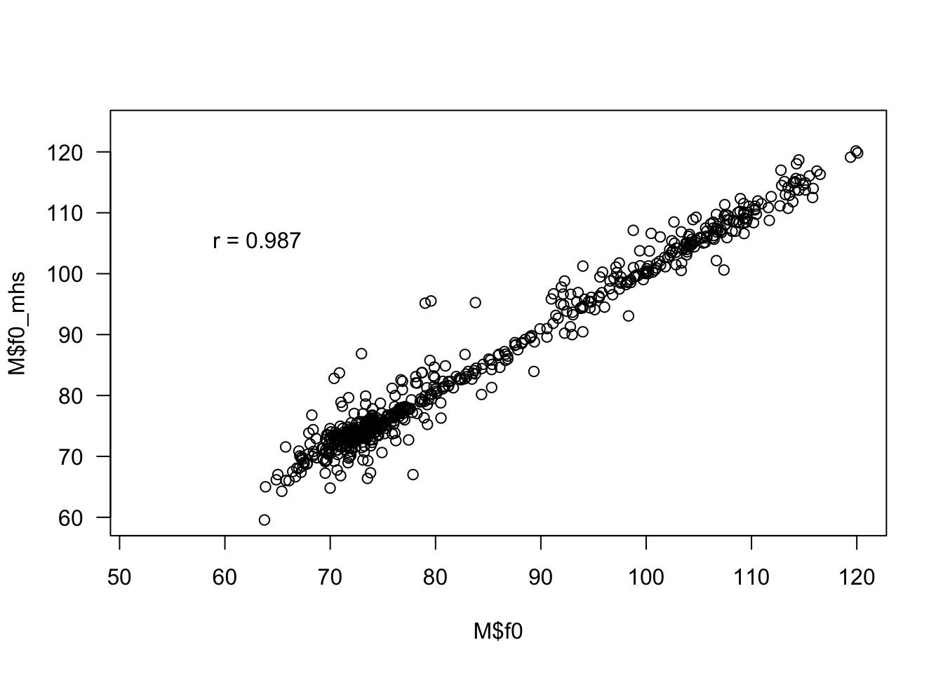
Exercise 7.1
- Review the documentation for the
anscombeobject.
- Access the links datasauRus e https://marcusnunes.me/posts/correlacoes-e-graficos-de-dispersao/. \(\\\)
Exercise 7.2 Access the link about Bivariate Correlation Simulation and Bivariate Scatter Plotting and carry out simulations varying the parameters, observing the resulting graphs.
7.1.1 \(\rho\) \(\cdot\) Universal correlation
(Samuel Kotz et al. 2005, 1375) define the universal correlation of two r.v. \(X\) and \(Y\) by \[\begin{equation} \rho = Cor(X,Y) = \dfrac{Cov(X,Y)}{D(X) D(Y)}, \tag{7.1} \end{equation}\] where \[\begin{equation} Cov(X,Y) = E \left[ (X-E(X)) (Y-E(Y)) \right] = \frac{\sum_{i=1}^N (x_{i} - \mu_{X})(y_{i} - \mu_{Y})}{N} \tag{7.2} \end{equation}\] is the covariance between \(X\) and \(Y\), \(D(X)\) and \(D(Y)\) are respectively the universal standard deviations of \(X\) and \(Y\) according to Eq. (2.26) e \[\begin{equation} -1 \le \rho \le +1 \end{equation}\] \[ \Updownarrow \] \[\begin{equation} 0 \le |\rho| \le +1. \end{equation}\]
If \(|\rho| = +1\), then there is a linear relationship of the form \(Y = \beta_0 + \beta_1 X\). If \(\rho = +1\), \(\beta_1 >0\); if \(\rho = -1\), \(\beta_1 <0\). If \(X\) is independent of \(Y\), then \(\rho = 0\), but the opposite is not necessarily true.
7.1.2 \(r\) \(\cdot\) Pearson Correlation Coefficient
The Pearson correlation coefficient was developed by Karl Pearson and William Fleetwood Sheppard “before the end of 1897”, as reported by (Pearson 1920, 44). Denoted by \(r\), it can be obtained by any of the following equations.
\[\begin{equation} r = \frac{1}{n-1} \sum_{i=1}^{n} \left( \dfrac{x_{i} - \bar{x}}{s_{x}} \right) \left( \dfrac{y_{i} - \bar{y}}{s_{y}} \right) \tag{7.3} \end{equation}\]
\[\begin{equation} r = \frac{\sum (x - \bar{x})(y - \bar{y})}{\sqrt{\sum (x - \bar{x})^2 \sum (y - \bar{y})^2}} \tag{7.4} \end{equation}\]
\[\begin{equation} r = \frac{n \sum{x y} - \sum{x} \sum{y}}{\sqrt{[n \sum{x^2} - (\sum{x})^2] [n \sum{y^2} - (\sum{y})^2]}} \tag{7.5} \end{equation}\]
where \[ \bar{x} = \frac{1}{n} \sum_{i=1}^{n} x_{i}, \;\; s_{x}^2 = \frac{1}{n-1} \sum_{i=1}^{n} (x_{i} - \bar{x}) ^2 \] \[ \bar{y} = \frac{1}{n} \sum_{i=1}^{n} y_{i}, \;\; s_{y}^2 = \frac{1}{n-1} \sum_{i=1}^{n} (y_{i} - \bar{y}) ^2 \] \[ -1 \le r \le +1 \]
Note from Equation (7.3) that \(r\) is an average of the products of the ordered pairs \((x_{i}, y_{i})\) standardized, with \(i \in \lbrace 1, 2 , \ldots, n \rbrace\). If positive product pairs predominate, \(r\) will be positive; if there is a predominance of negative product pairs, \(r\) will be negative. This structure is called product moment. The Equation (7.4) refers to the definition (7.1), while the Equation (7.5) is useful for carrying out the calculations.
Example 7.2 Consider the idea of estimating the number of beverage bottles to be chilled depending on the maximum temperature of the day. Let \(X\): ‘maximum temperature of the day in \(^{\circ}{\rm C}\)’ and \(Y\): ‘number of bottles of drink consumed’, observed according to the following table.
| \(i\) | \(x_{i}\) | \(y_{i}\) | \(i\) | \(x_{i}\) | \(y_{i}\) | \(i\) | \(x_{i}\) | \(y_{i}\) |
|---|---|---|---|---|---|---|---|---|
| 1 | 29.5 | 146 | 11 | 28.5 | 183 | 21 | 40.9 | 233 |
| 2 | 31.3 | 170 | 12 | 28.0 | 158 | 22 | 28.6 | 169 |
| 3 | 34.7 | 167 | 13 | 36.7 | 181 | 23 | 36.1 | 192 |
| 4 | 40.4 | 244 | 14 | 31.5 | 123 | 24 | 27.1 | 106 |
| 5 | 28.4 | 159 | 15 | 38.1 | 223 | 25 | 29.5 | 170 |
| 6 | 40.3 | 195 | 16 | 33.5 | 176 | 26 | 31.6 | 167 |
| 7 | 41.1 | 225 | 17 | 37.2 | 196 | 27 | 25.2 | 133 |
| 8 | 36.2 | 206 | 18 | 41.9 | 238 | 28 | 31.5 | 138 |
| 9 | 35.7 | 200 | 19 | 31.5 | 184 | 29 | 39.8 | 199 |
| 10 | 26.1 | 134 | 20 | 38.2 | 213 | 30 | 30.8 | 172 |
A scatter plot can help explore the behavior of temperature and bottles consumed.
dr <- read.table('https://filipezabala.com/data/drinks.txt', header = T)
dim(dr)  # dataset dimension
## [1] 30 2## temp gar
## 1 29.5 146
## 2 31.3 170
## 3 34.7 167
## 4 40.4 244
## 5 28.4 159
## 6 40.3 195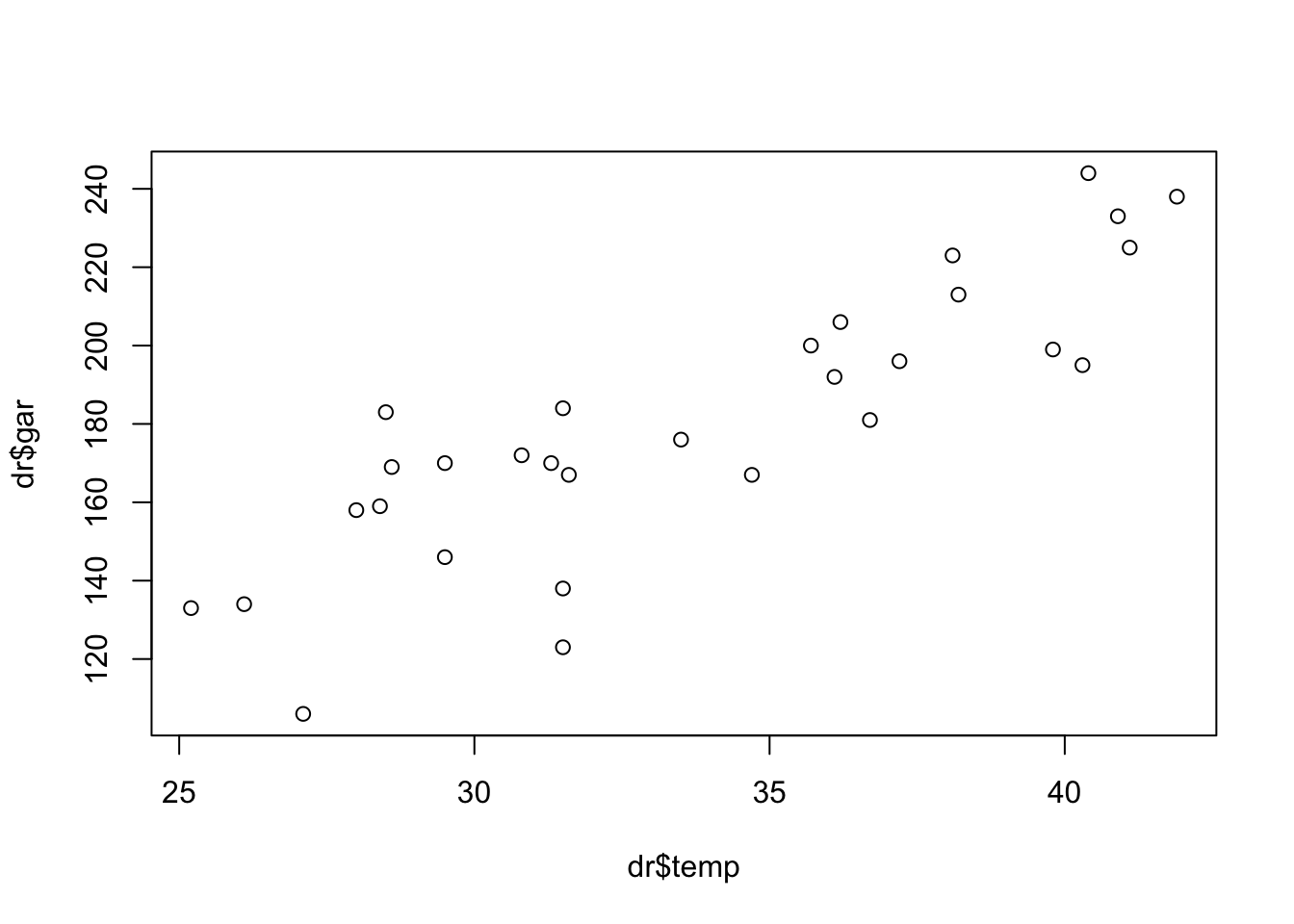
The degree of alignment of variables can be estimated by Pearson’s correlation coefficient, simply calculating \[ \sum{x} = 1010, \; \sum{x}^2 = 34730, \] \[ \sum{y} = 5400, \; \sum{y}^2 = 1006954, \] \[ \sum{x y} = 186117, \; n=30 \]
and replace in Equation (7.5), resulting in
\[\begin{equation} r = \frac{30 \times 186117 - 1010 \times 5400}{\sqrt{[30 \times 34730 - 1010^2] [30 \times 1006954 - 5400^2]}} \nonumber \\ r = \frac{130056}{\sqrt{21988.49 \times 1048620}} \nonumber \\ r \approx 0.8565. \nonumber \end{equation}\]
## [1] 0.8564926It is possible to obtain the value of \(r\) from the stats::lm function. It calculates the coefficient of determination \(r^2\) according to Section 7.1.4, which in the RLS model (Section 7.2) is the square of \(r\). Therefore \(r=\sqrt{r^2}\).
f <- lm(dr$gar ~ dr$temp)                   # SLR model
r2 <- summary(f)$r.squared                  # Extracting r2
sqrt(r2)                                    # r, Pearson correlation
## [1] 0.8564926## [1] TRUEExercise 7.3 Calculate the value of \(r\) with the data from Example 7.2 from Equations (7.3) and (7.4). Compare with the values obtained via Eq. (7.5) and the stats::cor function.
Test for \(\rho\)
The basic test is to compare \(\rho\) with zero, which indicates a complete lack of alignment between the variables. Thus, we test \(H_0: \rho = 0\) (there is no correlation) vs \(H_1: \rho \ne 0\) (there is correlation), denoted by
\[ \left\{ \begin{array}{l} H_0: \rho = 0 \\ H_1: \rho \ne 0\\ \end{array} \right. . \]
Under \(H_0\) considering the SLR model (Section 7.2), \[\begin{equation} T = \frac{r}{\sqrt{\frac{1-r^2}{n-2}}} \sim t_{n-2}. \tag{7.6} \end{equation}\]
Exercise 7.4 From Eq. (7.6), show that \(T = r \sqrt{\frac{n-2}{1-r^2}}\).
Example 7.3 (Checking alignment in the SLR model) Consider again the information presented in Example 7.2. Considering the model estimate \(y = -19.11 + 5.91 x\), one can test \(H_0: \rho = 0\) vs \(H_1: \rho \ne 0\). In this case \(gl=30-2=28\), \(T \sim t_{28}\) and under \(H_0\) \[ T = 0.8565 \sqrt{\frac{30-2}{1-0.8565^2}} \approx 8.78. \]
## [1] 0.8564926## [1] 8.780493## [1] 1.565265e-09##
## Pearson's product-moment correlation
##
## data: dr$temp and dr$gar
## t = 8.7805, df = 28, p-value = 1.565e-09
## alternative hypothesis: true correlation is not equal to 0
## 95 percent confidence interval:
## 0.7176748 0.9298423
## sample estimates:
## cor
## 0.8564926## [1] TRUECI for \(\rho\)
Step 1: Obtain Fisher’s z transformation (Ronald A. Fisher 1921, 210).
\[\begin{equation} z_r = \frac{1}{2} \ln \left( \frac{1+r}{1-r} \right) = \tanh^{-1}(r) \tag{7.7} \end{equation}\]
Step 2: Get the transformed lower and upper bounds with the desired confidence \(1-\alpha\).
\[\begin{equation} L = z_r - \frac{z_{1-\alpha/2}}{\sqrt{n-3}} \tag{7.8} \end{equation}\]
\[\begin{equation} U = z_r + \frac{z_{1-\alpha/2}}{\sqrt{n-3}} \tag{7.9} \end{equation}\]
Step 3: Obtain the confidence interval \(1-\alpha\) for \(\rho\).
\[\begin{equation} IC[\rho, 1-\alpha] = [ \frac{e^{2L}-1}{e^{2L}+1}, \frac{e^{2U}-1}{e^{2U}+1} ] = [ \tanh L, \tanh U ] \tag{7.10} \end{equation}\]
Example 7.4 Considering the data from Example 7.3 the 95% CI for the correlation can be obtained.
## [1] 1.280029## [1] 0.3772022## [1] 0.9028267## [1] 1.657231## [1] 0.7176715## [1] 0.9298433Exercise 7.5
- Check the identity of Equations (7.7) and (7.10). Apply the alternative equations to the data in Example 7.4 and compare with the output of the
stats::cor.testfunction.
- Get \(CI[ \rho, 80\% ]\).
- Write a function that returns the IC for \(\rho\) as a function of two vectors and an arbitrary confidence.
7.1.3 \(\rho_{RTO}\) and \(r_{RTO}\) \(\cdot\) Correlation in RTO
There is a special case of correlation calculation called Regression through the Origin (RTO), based on the model according to Eq. (7.17). In this case, \(r_{RTO}\) is calculated using the expression
\[\begin{equation} r_{RPO} = \sqrt{\dfrac{\sum \hat{y}_{i}^2}{\sum y_{i}^2}}, \tag{7.11} \end{equation}\]
such that \(\hat{y}_{i} = \hat{\beta}_1^{RPO}x_i\).
Example 7.5 (Correlation in RTO) Consider the information from Example 7.2. It can be calculated \[ r_{RTO} = \sqrt{\dfrac{997410}{1006954}} = \sqrt{0.9905} \approx 0.9952. \]
## [1] 0.9905222It is possible to obtain the value of \(r_{RTO}\) from the stats::lm function. It calculates the coefficient of determination \(r_{RTO}^2\), which in the RPO model is the square of \(r_{RTO}\). Therefore \(r_{RTO}=\sqrt{r_{RTO}^2}\).
f_rto <- lm(dr$gar ~ dr$temp - 1)         # RTO model
r2_rto <- summary(f_rto)$r.squared        # Function to get r2_RTO
sqrt(r2_rto)                              # r_RTO
## [1] 0.9952498## [1] TRUEExercise 7.6 Consider again the information presented in Example 7.2.
a. From the Example 7.9 it is known that \(\hat{y}_{i} = 5.36 x_i\), such that $x_i {29.5, 31.3, , 30.8 } $. Show that \(\sum \hat{y}_{i}^2 = 997410\).
b. Inspect the f$fitted.values object from Example 7.5.
Test for \(\rho_{RPO}\)
If we consider the RPO model according to Eq. (7.17), we can test the hypotheses
\[ \left\{ \begin{array}{l} H_0: \rho_{RTO} = 0 \\ H_1: \rho_{RTO} \ne 0\\ \end{array} \right. . \]
Under \(H_0\), the test statistic is \[\begin{equation} T_{RTO} = \frac{r_{RTO}}{\sqrt{\frac{1-r_{RTO}^2}{n-1}}} \sim t_{n-1}. \tag{7.12} \end{equation}\]
Example 7.6 (Checking alignment in the RTO model) Consider again the information presented in Example 7.2. If the RTO model estimate is \(y = 5.36 x\), one can test
\[ \left\{ \begin{array}{l} H_0: \rho^{RTO} = 0 \\ H_1: \rho^{RTO} \ne 0\\ \end{array} \right. \]
In this case \(df=30-1=29\), \(T \sim t_{29}\) and under \(H_0\) \[ T = 0.9952 \sqrt{\frac{30-1}{1-0.9952^2}} \approx 55.05. \]
## [1] 0.9952498## [1] 55.05267## [1] 6.778938e-31