2.1 Variables
The definitions of (Agresti and Franklin 2013, 25) are considered.
Definition 2.1 A variable is any characteristic observed in a study.
Definition 2.2 A variable is called qualitative or categorical if each observation belongs to one of a set of categories.
Definition 2.3 A variable is called quantitative or numerical if observations on it take numerical values that represent different magnitudes of the variable.
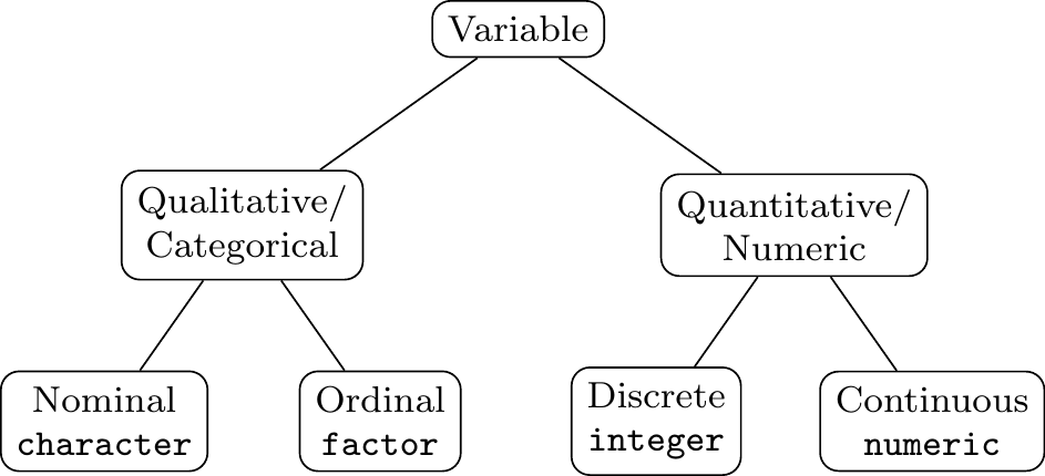
Figure 2.1: A possible classification of variables.
2.1.1 Nominal scale
Qualitative nominal scale variables have the lowest degree of information among the four proposed types, allowing only the evaluation of frequencies and arbitrary ordering. They are applied in evaluations of unordered groups, such as ‘sex’, ‘religion’, ‘race’, ‘preferred color’, ‘neighborhood where you live’, ‘soccer team you love’, etc.
2.1.2 Ordinal scale
Qualitative ordinal scale variables have a higher degree of information in relation to the nominal ones because they are endowed with a previous ordering, allowing comparisons between the observations. Variables of an ordinal nature evaluate ordered groups, such as ‘placement in a sports tournament’, ‘education level’, ‘ranking of a restaurant in terms of food quality’, etc.
Example 2.1 (Placement in the entrance exam) The variable ‘general placement in the entrance exam’ is classified as ordinal because it indicates the ordering of the entrance exam in comparison to the others, even if the final grade of each candidate is not known.
Example 2.2 (Likert Scale) When you want to measure the degree of satisfaction with a good or service, you can use the Likert Scale of \(k\) levels proposed by (Likert 1932). One advantage of using even \(k\), is that the respondent is forced to position himself in favor/against, above/below.
If \(k=4\),
1: Bad, 2: Fair, 3: Good, 4: Excellent.
If \(k=5\),
1: Bad, 2: Bad, 3: Fair, 4: Good, 5: Excellent. \(\\\)
Example 2.3 (Knuth Scale) (Knuth 1968, xvii-xviii) suggests a scale from 0 to 50 to rank exercises by their degree of difficulty. For this he considers the principle stated by Richard Bellmann:
If you can solve it, it is an exercise; otherwise it is a research problem.
For this he proposes interpretations for some ratings of reference.
00 An extremely easy exercise which can be answered immediately if the material of the text has been understood, and which can almost always be worked “in your head.”
10 A simple problem, which makes a person think over the material just read, but which is by no means difficult. It should be possible to do this in one minute at most; pencil and paper may be useful in obtaining the solution.
20 An average problem which tests basic understanding of the text material but which may take about fifteen to twenty minutes to answer completely.
30 A problem of moderate difficulty and/or complexity which may involve over two hours’ work to solve satisfactorily.
40 Quite a difficult or lengthy problem which is perhaps suitable for a term project in classroom situations. It is expected that a student will be able to solve the problem in a reasonable amount of time, but the solution is not trivial.
50 A research problem which (to the author’s knowledge at the time of writing) has not yet been solved satisfactorily. If the reader has found an answer to this problem, he is urged to write it up for publication; furthermore, the author of this book would appreciate hearing about the solution as soon as possible. (Erdős and Spencer 1974) offered prizes in the order of US$25 for solving problems of this class.
Summarizing ordinal variables
Ordinal data inform the order of observations, not their magnitude. Thus, to summarize ordinal data, it is recommended to use median (Eq. (2.17)), interquartile range (Eq. (2.28)) and median absolute deviation (Eq. (2.29)).
Exercise 2.1 (Rubio-Rivas et al. 2022) present a comparative study of ordinal severity scales proposed by the World Health Organization. Access the article available at this link and check how the data was summarized.
2.1.3 Discrete
A discrete quantitative variable in short assumes only integer values. Technically, discrete variables are characterized by countable sets.
Example 2.4 (Number of children) Suppose you want to observe the number of children of women assisted in a hospital. For each woman interviewed, the set of possible answers to the question ‘how many children do you have?’ is \(C = \lbrace 0, 1, 2, \ldots, k \rbrace\), where \(k\) is the maximum number of children a woman can have in her lifetime. According to the Guinness Book of Records the world record is \(k=69\), attributed to Russian Valentina Vassilyeva. On four occasions she gave birth to quadruplets (16), seven to triplets (21) and sixteen to twins (32). This is a finite countable set. \(\\\)
Example 2.5 (Points on a die thrown \(k\) times) Suppose \(k\) die rolls. In each throw, the resulting face is noted, added to the values obtained in the \(k-1\) previous rolls. The set of possible outcomes of this experiment is \(S = \lbrace k, k+1, \ldots, 6k \rbrace\). This is a finite countable set. As an exercise, do \(k=4\) and reread the previous sentence substituting the values. \(\\\)
Example 2.6 (Eternal consumption engine) Suppose an eternal consumption engine, measured in steps. The set of possible number of steps is \(S = \lbrace 1, 2, \ldots \rbrace\). This is an infinitely countable set. \(\\\)
Example 2.7 (Pilcher’s Squad) Norman Pilcher was the creator of the Drug Squad, and gained notoriety in the 60s for arresting artists like Mick Jagger and John Lennon. The set of artists Sergeant Pilcher could arrest is \(A = \lbrace a_{1}, a_{2}, \ldots, a_{k} \rbrace\), where \(k\) represents the number of artists available to be arrested. This is a finite countable set. \(\\\)
2.1.4 Continuous
The continuous quantitative variable is characterized by allowing the observation of any subset of real numbers as a result. It is used to evaluate time, distances, areas, volumes or any other non-countable numeric quantity. As with discrete variables, it is possible to assess mathematical relationships between observed values.
Example 2.8 (Proportion of people who wear glasses) Suppose a group of researchers is interested in assessing the ‘proportion of people who wear glasses in a university’. This value must be between 0 and 1 (or 0% and 100%), and can be represented by the uncountable set \(\Omega = \lbrace b \in \mathbb{R} : 0 \le b\le 1 \rbrace\). \(\\\)
Example 2.9 (Age) The ‘age’ variable is classified as continuous because it represents a temporal notion. The set of possible lifetimes of a human being is given by \(\Omega = \lbrace t \in \mathbb{R} : 0 \le t \le T \rbrace\), where \(T\) is the maximum age in years that a human being can achieve. According to the Guinness Book of Records, the Gerontology Research Group and a Gerontology Wiki, \(T \approx 122.45015298055400876365\), achieved by Frenchwoman Jeanne Louise Calment. Calment was born on 02/21/1875 and died on 08/04/1997. \(\Omega\) is said to be uncountable since it is not possible to count its number of elements. \(\\\)
## Time difference of 44724 days## [1] "122.45015298055400876365"Example 2.10 (Going down the level) Suppose a group of people was evaluated in relation to the variable ‘age’ measured in years, considering the hour and minute of birth. It is possible to transform it into the ‘discrete age’ variable simply by truncating the observed values. Likewise, it can be transformed into the ‘ordinal age’ variable, classifying it according to the following table.
| i | Age group | Group |
|---|---|---|
| 1 | Up to 10 years | Child |
| 2 | 10 \(\vdash\) 13 | Preteen |
| 3 | 13 \(\vdash\) 18 | Adolescent |
| 4 | 18 \(\vdash\) 35 | Young adult |
| 5 | 35 \(\vdash\) 45 | Adult |
| 6 | 45 \(\vdash\) 65 | Mature adult |
| 7 | 65 \(\vdash\) 75 | Young elderly |
| 8 | 75 + | Elderly |
Note that if a person is 31.99 years old (continuous), one can consider the truncated age of 31 years old (discrete) and classify this person as a ‘young adult’ (ordinal). However, given that a person is classified as a young adult, it is only possible to state that he/she is aged between 18 years (completed) and 35 years (incomplete) according to the proposed classification. \(\\\)
2.1.5 Final remarks
Each type of variable presents a level of information that must be respected. It is possible to go from a higher ranking level to a lower ranking level, but never the other way around. It is worth remembering that information is lost when the variable classification level is lowered. It is quite common, however, to find works using inappropriate classification levels, leading to inappropriate techniques that lead to wrong conclusions.
Exercise 2.2 Classify the variables below (qualitative nominal/ordinal, quantitative discrete/continuous).
- Number of refrigerators at home
- Pool water temperatures on a summer day
- Number of suicides in a city over the past year
- Lead concentration in a water sample
- List of book publishers
- Degree of satisfaction of customers who attend a cockfight
- Fabric softener brands
- Time a patient survives after a given diagnosis
- Market share (market share)
- Ranking in a bathtub race
- End time of each runner
- List of participating hot tub names, such as ‘Dick Dastardly’ and ‘Trollface’
- Distance from Istanbul to Rio de Janeiro
Suggestion: Chapter 8