3.5 Law of Total Probability and Bayes’ Theorem
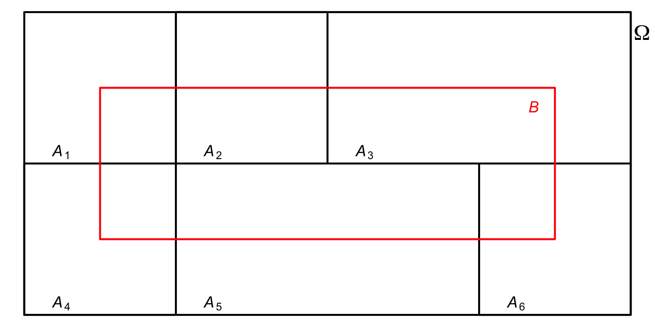
Figure 3.1: \(\Omega\) partition.
Consider a partition according to the Venn diagram of the figure above, where \(A_1, \ldots, A_5\) form a probability distribution, i.e., \(\sum_{i=1}^{5} Pr(A_i) =1\). One can decompose \(B\) as follows: \[\begin{equation} B = \cup_{i=1}^{5} (A_i \cap B) \end{equation}\]
Theorem 3.1 (Law of Total Probability) Let be an enumerable sequence of random events \(A_{1}, A_{2}, \ldots, A_{k}\), forming a partition of \(\Omega\). Since the intersections \(A_i \cap B\) are mutually exclusive, then from (3.23)
\[\begin{equation} Pr(B) = \sum_{i=1}^k Pr(A_i \cap B) \tag{3.40} \end{equation}\]
Applying (3.34), we can write
\[\begin{equation} Pr(B) = \sum_{i} Pr(A_{i}) \cdot Pr(B|A_{i}) \tag{3.41} \end{equation}\]
\(\bigtriangleup\)
From (3.32) one can calculate the probability of \(A_{i}\) given the occurrence of \(B\) by
\[\begin{equation} Pr(A_{i}|B) = \dfrac{Pr(A_{i} \cap B)}{Pr(B)} \tag{3.42} \end{equation}\]
Applying (3.41) in the denominator and (3.34) in the numerator of (3.42), \[\begin{equation} Pr(A_{i}|B) = \dfrac{Pr(A_{i}) \cdot Pr(B|A_{i})}{\sum_{j} Pr(A_{j}) \cdot Pr(B|A_{j})} \tag{3.43} \end{equation}\]
This is the Bayes Theorem (Bayes 1763), useful when we know the conditional probabilities of \(B\) given \(A_{i}\), but not directly the probability of \(B\). For a discussion of inverse probability, see Chapter 3 of (Stigler 1986).
Example 3.20 Consider the data from Example 1.2. It is possible to calculate \(Pr(D|T)\). \[\begin{align*} Pr(D|T) =& \frac{Pr(D) \cdot Pr(T|D)}{Pr(D) \cdot Pr(T|D) + Pr(\bar{D}) \cdot Pr(T|\bar{D})} \\ =& \frac{0.1 \times 1}{0.1 \times 1 + 0.9 \times 0.1} \\ =& \frac{10}{19} \\ Pr(D|T) \approx& 0.5263 \\ \end{align*}\]
Example 3.21 (Bayes’ Theorem) Suppose a box contains three coins, one balanced18 and two with two heads. The conditional probability that the coin drawn was the balanced one can be calculated. For that, you can define \(A_{1}:\) ‘the withdrawn coin is balanced’, \(A_{2}:\) ‘the withdrawn coin has two heads’ and \(B:\) ‘the final result is heads’ and apply the Bayes rule, resulting in \[ Pr(A_{1}|B) = \dfrac{Pr(A_{1}) \cdot Pr(B|A_{1})}{Pr(A_{1}) \ cdot Pr(B|A_{1}) + Pr(A_{2}) \cdot Pr(B|A_{2})} = \dfrac{\frac{1}{3} \times \frac{1}{ 2}}{\frac{1}{3} \times \frac{1}{2} + \frac{2}{3} \times 1} = \frac{1}{5} = 0.2. \]
## [1] 0.2Exercise 3.9 Obtain \(Pr(A_{2}|B)\) from Eq. (3.43) and verify that \(Pr(A_{2}|B) = 1-Pr(A_{1}|B)\).
Exercise 3.10 Consider a test where the probability of a false positive is 2% and the probability of a false negative is 5%. If a disease has a 1% prevalence in the population, what is the probability that a person has the disease if the test is positive?
Exercise 3.11 Read the summary and do the exercises in Chapter 2 of Probability Exercises by professor Élcio Lebensztayn.
References
Technical term indicating that each coin has a head and a tail, both with probability \(\frac{1}{2}\) of occurrence.↩︎