7.2 Simple Linear Regression
7.2.1 Model
The population/universal Simple Linear Regression (SLR) model is constructed, in the classical approach, with all \(N\) ordered pairs of the population or universe, i.e., \((x_i,y_i), \; i \in \{1,\ldots,N\}\). It can be described by Eq. (7.13).
\[\begin{equation} Y = \beta_0 + \beta_1 x + \varepsilon, \tag{7.13} \end{equation}\] where \(\varepsilon \sim \mathcal{N}(0,\sigma_{\varepsilon})\).
Note that for simplicity we consider \(Y \equiv Y_i\), \(x \equiv x_i\) and \(\varepsilon \equiv \varepsilon_i\). It is also important to keep in mind that the random variable \(Y\) represents the expectation conditional on the observed values of \(x\), denoted by \(E(Y|x)\). The estimate of \(E(Y|x) = Y\) will be noted by \(\widehat{E(Y|x)} = y\).
Example 7.7 In the following graph you can see that the blue line refers to the average \(\bar{y}=180\). This value is constant – or unconditional – for any value of \(x\) (in this case the maximum temperature of the day on the Celsius scale). The dotted red line indicates that a low value of \(y\) (in this case the number of bottles sold on the day) is expected the lower the \(x\), and a high \(y\) the higher the \(x\).
plot(dr$temp, dr$gar, las = 1)
abline(h = mean(dr$gar), col = 'blue')
abline(a = -19.11, b = 5.91, col = 'red', lty = 2)
legend(26, 235, legend=c('Unconditional','Conditional'),
       col = c('blue', 'red'), lty = 1:2, cex = 0.8, box.lty = 0)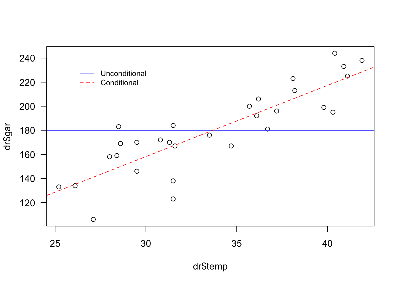
Parameter estimation
In most practical cases we work with samples, making it necessary to estimate the values of \(\beta_0\) and \(\beta_1\). The least squares method can be used to calculate these estimates. The principle of the method is to minimize the sum of squared errors, i.e., \[\begin{equation} \text{minimize} \sum_{i=1}^n \varepsilon_{i}^{2}. \tag{7.14} \end{equation}\]
Basically, \(\varepsilon = Y - \beta_0 - \beta_1 x\) from Eq. (7.13) is used and derived (partially) in relation to \(\beta_0\) and \(\beta_1\), making each one of the partial derivatives equal to zero. For more details, (DeGroot and Schervish 2012, 689) is recommended. The least squares estimates are finally given by
\[\begin{equation} \hat{\beta}_1 = \frac{n \sum{xy} - \sum{x} \sum{y}}{n \sum{x^2} - (\sum{x})^2} \tag{7.15} \end{equation}\] and \[\begin{equation} \hat{\beta}_0 = \bar{y} - \hat{\beta}_1 \bar{x}. \tag{7.16} \end{equation}\]
Example 7.8 Consider again the data from Example 7.2. A simple linear model can be adjusted according to Equations (7.13), (7.15) and (7.16). Note the estimate in the form \(y = -19.11 + 5.91 x\).
##
## Call:
## lm(formula = gar ~ temp, data = dr)
##
## Coefficients:
## (Intercept)         temp
##     -19.110        5.915
RTO model
A model in the form of Eq. (7.17) is called Regression Through Origin (RTO) because the fitted line passes through the point \((0,0)\), the origin of the Cartesian plane. Just do \(\beta_0=0\) in Equation (7.13), and for more details see (Eisenhauer 2003). \[\begin{equation} Y = \beta_1^{RTO} x + \varepsilon, \tag{7.17} \end{equation}\] onde \(\varepsilon \sim \mathcal{N}(0,\sigma_{\varepsilon})\). A estimativa do parâmetro \(\beta_1^{RTO}\) é dada por \[\begin{equation} \hat{\beta}_1^{RTO} = \frac{\sum{xy} }{\sum{x^2}}. \tag{7.18} \end{equation}\]
Example 7.9 Consider again the data from Example 7.2. An RTO model can be adjusted according to Equations (7.17) and (7.18), resulting in \(y = 5.36 x\). In the R function stats::lm (linear model) it is possible to make the adjustment using + 0 instead of - 1.
##
## Call:
## lm(formula = gar ~ temp - 1, data = dr)
##
## Coefficients:
##  temp
## 5.359
Exercise 7.7 Consider again the data from Examples 7.2 and 7.8.
a. Calculate by hand the estimate of the parameters of the model described in Equation (7.13) considering Equations (7.15) and (7.16).
b. Calculate by hand the estimate of the parameters of the model described in Equation (7.17) considering Equation (7.18).
\(\\\)
7.2.2 Inferential diagnostics
Inferential analysis consists of evaluating the quality of a model in relation to the estimation of its parameters (\(\theta\)). In this way, we can think from the perspective of understanding the model. This understanding usually involves evaluating the model’s adherence to the data, assigning degrees of evidence to hypotheses associated with the modeled parameters or minimizing some theoretical information criterion.
Test for \(\beta_0\)
The usual test hypotheses for \(\beta_0\) are \(H_0: \beta_0 = 0\) vs \(H_1: \beta_0 \ne 0\). Under \(H_0\) \[\begin{equation} T_0 = \frac{\hat{\beta}_0}{se(\hat{\beta}_0)} \sim t_{n-2}, \tag{7.19} \end{equation}\] where \(\hat{\beta}_0\) is given by Eq. (7.16) and \[\begin{equation} se(\hat{\beta}_0) = \sqrt{\hat{\sigma}^2 \left[ \frac{1}{n} + \frac{\bar{x}^2}{S_{xx}} \right] } = \sqrt{\frac{\sum_{i=1}^n (y_i - \hat{y}_i)^2}{n-2} \left[ \frac{1}{n} + \frac{\bar{x}^2}{\sum_{i=1}^n (x_i - \bar{x})^2} \right] }. \tag{7.20} \end{equation}\]
Test for \(\beta_1\)
Testing for \(\beta_1\) is fundamental in diagnostic analysis. It is with him that one decides regarding the presence or absence of a linear relationship between \(X\) and \(Y\). The usual test hypotheses for \(\beta_1\) are \(H_0: \beta_1 = 0\) vs \(H_1: \beta_1 \ne 0\). Under \(H_0\) \[\begin{equation} T_1 = \frac{\hat{\beta}_1}{se(\hat{\beta}_1)} \sim t_{n-2}, \tag{7.21} \end{equation}\] onde \(\hat{\beta}_1\) is given by Eq. (7.15) and \[\begin{equation} se(\hat{\beta}_1) = \sqrt{\frac{\hat{\sigma}^2}{S_{xx}}} = \sqrt{\frac{\sum_{i=1}^n (y_i - \hat{y}_i)^2 / (n-2)}{\sum_{i=1}^n (x_i - \bar{x})^2} }. \tag{7.22} \end{equation}\]
Test for \(\beta_1^{RTO}\)
\[\begin{equation} T_1^{RTO} = \frac{\hat{\beta}_1^{RTO}}{se(\hat{\beta}_1^{RTO})} \sim t_{n-1}, \tag{7.23} \end{equation}\] where \(\hat{\beta}_1^{RTO}\) is given by Eq. (7.18) and \[\begin{equation} se(\hat{\beta}_1^{RTO}) = \sqrt{\frac{\hat{\sigma}^2}{S_{xx}}} = \sqrt{\frac{\sum_{i=1}^n (y_i - \hat{y}_i)^2 / (n-1)}{\sum_{i=1}^n x_{i}^{2} } }. \tag{7.24} \end{equation}\]
Information criteria
AIC - Akaike Information Criterion
(Akaike 1974) proposes an information theoretical criterion according to Eq. (7.25). The lower the value of the measure, the better (in the sense of more parsimonious) the model.
\[\begin{equation} \text{AIC} = -2 l(\hat{\beta}) + 2n_{par}, \tag{7.25} \end{equation}\]
where \(n_{par}\) indicates the number of independently adjusted parameters in the model and \(l(\hat{\beta})\) is the logarithm of the maximum likelihood value of the model. For more details see ?stats::AIC and ?stats::logLik.
BIC - Critério de Informação Bayesiano
(Schwarz 1978) proposes an information theoretical criterion according to Eq. (7.26). The author argues26 that both AIC and BIC provide a mathematical formulation of the principle of parsimony in model construction. However, for a large number of observations, the two criteria may differ significantly from each other, making it more appropriate to give preference to BIC.
\[\begin{equation} \text{BIC} = -2 l(\hat{\beta}) + \log(n) n_{par}, \tag{7.26} \end{equation}\]
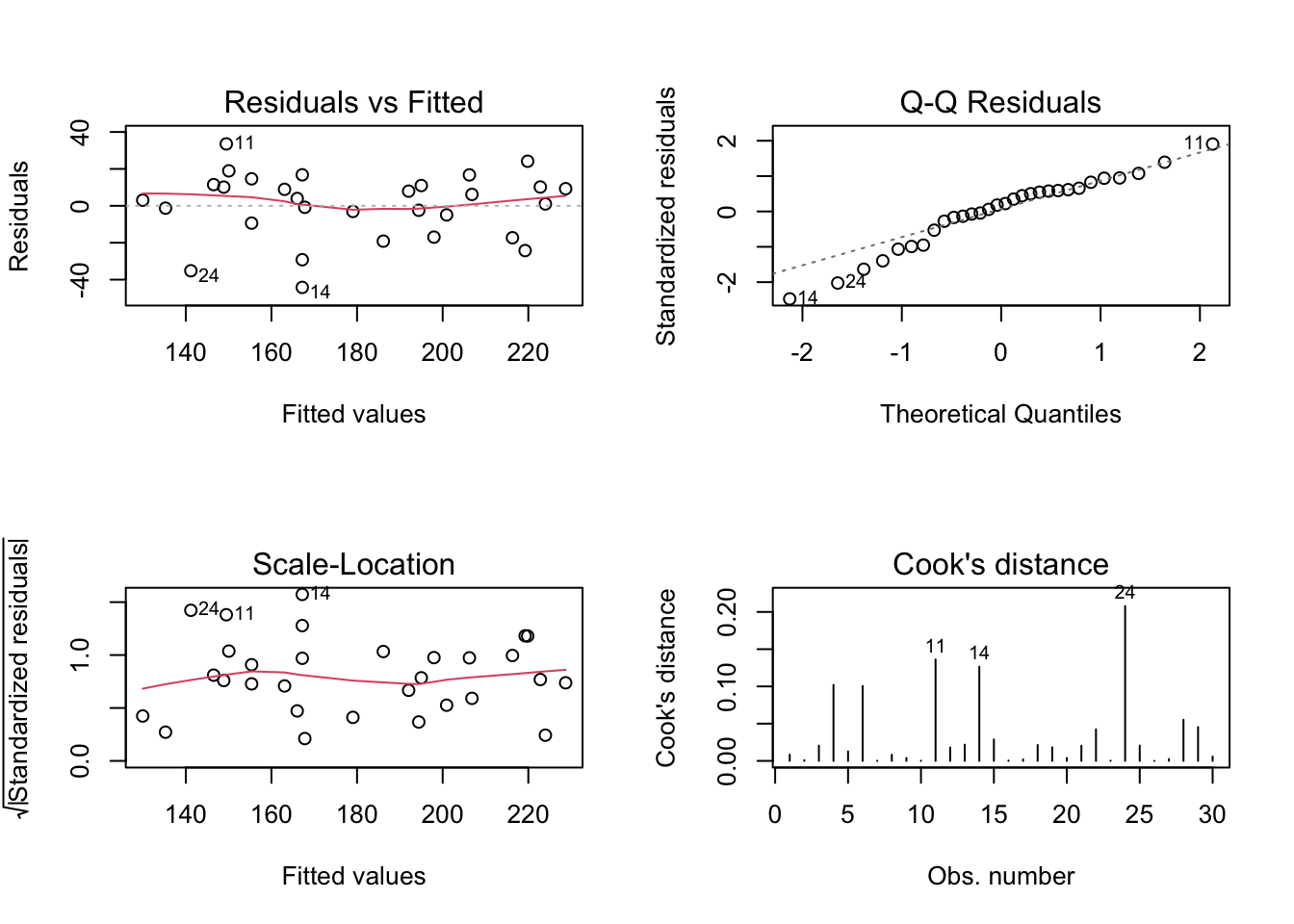
Example 7.10 Consider the Example 7.8. You can use R’s generic base::summary function to diagnose the models considered. The RLS model in the form \(y=-19.110+5.915x\) was assigned to the fit object.
##
## Call:
## lm(formula = gar ~ temp, data = dr)
##
## Residuals:
## Min 1Q Median 3Q Max
## -44.204 -8.261 3.518 10.796 33.540
##
## Coefficients:
## Estimate Std. Error t value Pr(>|t|)
## (Intercept) -19.1096 22.9195 -0.834 0.411
## temp 5.9147 0.6736 8.780 1.57e-09 ***
## ---
## Signif. codes: 0 '***' 0.001 '**' 0.01 '*' 0.05 '.' 0.1 ' ' 1
##
## Residual standard error: 18.24 on 28 degrees of freedom
## Multiple R-squared: 0.7336, Adjusted R-squared: 0.7241
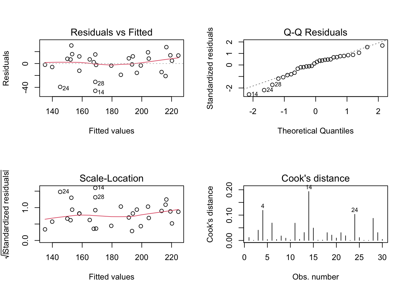
## F-statistic: 77.1 on 1 and 28 DF, p-value: 1.565e-09The RTO model in the form \(y=5.3590x\) was assigned to the fit0 object.
##
## Call:
## lm(formula = gar ~ temp - 1, data = dr)
##
## Residuals:
##     Min      1Q  Median      3Q     Max
## -45.810 -10.537   3.503  11.979  30.267
##
## Coefficients:
##      Estimate Std. Error t value Pr(>|t|)
## temp  5.35904    0.09734   55.05   <2e-16 ***
## ---
## Signif. codes:  0 '***' 0.001 '**' 0.01 '*' 0.05 '.' 0.1 ' ' 1
##
## Residual standard error: 18.14 on 29 degrees of freedom
## Multiple R-squared:  0.9905, Adjusted R-squared:  0.9902
## F-statistic:  3031 on 1 and 29 DF,  p-value: < 2.2e-16
The Akaike (AIC) and Schwartz (BIC) information criteria can be calculated respectively via stats::AIC and stats::BIC. The two criteria suggest that the RPO model is more parsimonious than the RLS model.
## [1] 263.2736## [1] 267.4772## [1] 262.0094## [1] 264.8118A visual inspection can also be carried out as a complement to the inferential analysis. For a well-adjusted model, it is expected that the residual graphs for adjusted values (first column) do not indicate any type of trend or modelable behavior. It is also expected for a good fit that the ‘Normal Q-Q’ graph presents the points as close as possible to the dotted line, which indicates perfect normality of the residuals. Cook’s distance from the last graph indicates possible influence points, which may be contributing disproportionately to the model. For more details see the documentation of ?stats::lm.influence, (R. D. Cook 1977) and (Paula 2013).
Exercise 7.9 Considering the Example 7.10, check:
a. \(\hat{\beta}_0 = -19.110\).
b. \(\hat{\beta}_1 = 5.915\).
c. \(se(\hat{\beta}_0) = 22.919\).
d. \(se(\hat{\beta}_1) = 0.674\).
e. \(T_0=-0.83\).
f. \(T_1=8.78\).
g. The p-value associated with the hypothesis \(H_0:\beta_0=0\) is \(0.41\).
h. The p-value associated with the hypothesis \(H_0:\beta_1=0\) is \(1.6e-09\).
i. \(\hat{\beta}_1^{RPO} = 5.3590\).
j. \(se(\hat{\beta}_1^{RPO}) = 0.0973\).
k. \(T_1^{RPO} = 55\).
l. The p-value associated with the hypothesis \(H_0:\beta_1^{RPO}=0\) is \(<2e-16\).
Example 7.11 Consider again the data from Example 7.1.
a. Regress M\(f0 by M\)f0_mhs and vice versa.
b. What do you notice after evaluating the summary of the models?
Exercise 7.10 Consider again the data from Example 7.2.
a. Perform the test of the model parameters described in Equation (7.13) by hand considering Equations (7.19), (7.20), @ref(eq :teste-b1) and (7.22).
b. Perform the test of the model parameters described in Equation (7.17) by hand considering Equations (7.23) and (7.24).
7.2.3 Predictive diagnostics
The predictive analysis consists of evaluating the quality of the model in relation to its ability to predict new values (\(X\)). In this way, we can think through the prism of the predictive capacity of the model. Such capacity can be assessed by several measures, depending on the type of variable involved.
Categorical variables typically require to be grouped or classified, and to measure the predictive capacity, measures such as accuracy, sensitivity, sensitivity, etc. are used. For more details see the documentation for ?caret::confusionMatrix and this Wikipedia article.
Models for numerical variables typically make use of the mean squared (prediction) error, or EQM, given by Eq. (7.27).
\[\begin{equation} \text{MSE} = \frac{\sum_i^{n} (y_i - \hat{y}_i)^2}{n} \tag{7.27} \end{equation}\]
You can write a function to calculate the MSE.
Example 7.12 Consider again the data from Example 7.2. Using the idea of training-testing, models can be compared in terms of their NDEs. To achieve this, \(M=100\) replications are carried out by adjusting the RLS and RPO models with \(ntrain=20\) training observations, compared with the remaining \(ntest=10\) test observations. Note that the sample draw is carried out using the base::sample function associated with sed.seed indexed by i, allowing exact replication of the results.
M <- 100          # Number of repetitions
ntrain <- 20      # Training sample size
fit_mse <- vector(length = M)   # Vector to store M MSEs from fit
fit0_mse <- vector(length = M)  # Vector to store M MSEs from fit

for(i in 1:M){
  set.seed(i); itrain <- sort(sample(1:nrow(dr), ntrain))
  train <- dr[itrain,]
  test <- dr[-itrain,]
  xtest <- data.frame(temp = dr[-itrain,'temp'])
  fit_temp <- lm(gar ~ temp, data = train)
  fit0_temp <- lm(gar ~ temp-1, data = train)
  fit_mse[i] <- mse(test$gar, predict(fit_temp, xtest))
  fit0_mse[i] <- mse(test$gar, predict(fit0_temp, xtest))
}
You can compare model NDEs numerically using the generic function base::summary and visually using graphics::boxplot.
##    Min. 1st Qu.  Median    Mean 3rd Qu.    Max.
## 145.9 301.4 362.1 386.7 455.0 815.2## Min. 1st Qu. Median Mean 3rd Qu. Max.
## 137.8 271.6 349.6 365.4 453.6 779.3
It is noted that the MSE values associated with the RTO fit0 model are slightly lower than those of the SLR fit model. In this way, the use of RTO is suggested to the detriment of SLR, even though the Student and Mann-Whitney tests (with their basic assumptions duly admitted) suggest that there is no significant difference between the means and medians of the MSEs of the models evaluated.
##
##  Welch Two Sample t-test
##
## data:  fit_mse and fit0_mse
## t = 1.1401, df = 197.99, p-value = 0.2556
## alternative hypothesis: true difference in means is not equal to 0
## 95 percent confidence interval:
##  -15.56988  58.24303
## sample estimates:
## mean of x mean of y
## 386.7044 365.3678##
## Wilcoxon rank sum test with continuity correction
##
## data: fit_mse and fit0_mse
## W = 5445, p-value = 0.2774
## alternative hypothesis: true location shift is not equal to 0References
Qualitatively both our procedure and Akaike’s give “a mathematical formulation of the principle of parsimony in model building.” Quantitatively, since our procedure differs from Akaike’s only in that the dimension is multiplied by \(\frac{1}{2}\log n\), our procedure leans more than Akaike’s towards lower-dimensional models (when there are 8 or more observations). For large numbers of observations the procedures differ markedly from each other. If the assumptions we made in Section 2 are accepted, Akaike’s criterion cannot be asymptotically optimal. This would contradict any proof of its optimality, but no such proof seems to have been published, and the heuristics of Akaike [1] and of Tong [4] do not seem to lead to any such proof.↩︎