6.3 Hypothesis Testing
Exercise 6.9 Check the hypothesis that the word ‘hypothesis’ comes from the Greek hypo (weak) + thesis = weak thesis as suggested by Renato Janine Ribeiro in Provoca on 24/08/2021.
Suggestion: Chapter 8
\(\\\)
6.3.1 Via confidence intervals
Hypothesis tests have the same characteristics and properties as their respective confidence intervals. Therefore, a brief example is presented addressing the equivalence between TH and IC for the universal proportion \(\pi\).
Example 6.11 (TH \(\equiv\) IC) Suppose a coin with probability of heads \(Pr(H)=\pi\). In principle we do not know the value of \(\pi\), and it may be interesting to consider two configurations:
\[\left\{ \begin{array}{l} H_0: \mbox{the coin is balanced}\\ H_1: \mbox{the coin is not balanced}\\ \end{array} \right. \equiv \left\{ \begin{array}{l} H_0: \pi = 0.5 \\ H_1: \pi \ne 0.5 \\ \end{array} \right. \]
Applying Charles Sanders Peirce idea of assuming \(H_{0}\) true (or ‘under \(H_{0}\)’), we expect to observe ‘heads’ in 50% of the results, with some variation around 50%. Considering Equation (6.4) one can obtain the expected margin of error for this oscillation depending on the sample size \(n\) for, say, 95% of cases: \[ IC \left[ \pi, 95\% \right] = 0.5 \mp 1.96 \sqrt{\dfrac{0.5 \left(1-0.5\right)}{n}} = 0.5 \mp \dfrac{0.98}{\sqrt{n} } \]
Thus, when performing \(n=25\) flips and observing a frequency of heads in the interval \[ IC \left[ \pi, 95\% \right] = 0.5 \mp \dfrac{0.98}{\sqrt{25}} = \left[ 0.304,0.696 \right] = \left[ 30.4\%,69.6\% \right] \] the coin can be considered balanced with \(1-\alpha=95\%\) confidence. If the frequency is lower than \(30.4\%\) or higher than \(69.6\%\), there is evidence that the currency is unbalanced, also with 95% confidence. According to hypothesis testing terminology, \(H_{0}\) is not rejected with \(\alpha=5\%\). If \(n=100\), \[ IC \left[ \pi, 95\% \right] = 0.5 \mp \dfrac{0.98}{\sqrt{100}} = \left[ 0.402,0.598 \right] = \left[ 40.2\%,59.8\% \right] \] and a smaller interval is obtained compared to \(n=25\), i.e., more accurate for the same 95% confidence. If As an exercise, use the function to set other values for \(n\) and test this result on a coin.
# 95% CI under H0: \pi=0.5
ic <- function(n){
   cat('[', 0.5-.98/sqrt(n), ',',
            0.5+.98/sqrt(n), ']')
}
ic(25)
## [ 0.304 , 0.696 ]## [ 0.402 , 0.598 ]6.3.3 Parametric space
Let a parameter \(\theta\) belong to a parameter space \(\Theta\), i.e., the set of all possible values of \(\theta\). Consider a partition such that \(\Theta_0 \cup \Theta_1 = \Theta\) and \(\Theta_0 \cap \Theta_1 = \emptyset\). A hypothesis test is a decision rule that allows you to decide, in light of the available information, whether it is more likely to admit \(\theta \in \Theta_0\) or \(\theta \in \Theta_1\). The hypothesis involving \(\Theta_0\) is called the null hypothesis, and the one involving \(\Theta_1\) is the alternative hypothesis. Such hypotheses can be written in the form
\[\left\{ \begin{array}{l} H_0: \theta \in \Theta_0\\ H_1: \theta \in \Theta_1 \\ \end{array} \right. \]
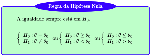
6.3.4 Null hypothesis \(H_0\)
Usually in hypothesis testing procedures it is initially assumed that \(H_0\) is true, said under the null hypothesis. For this reason, the null hypothesis must always contain equality, as indicated in the table below. Note that there is no ‘null hypothesis rule’, the indication is stated this way for didactic reasons only.
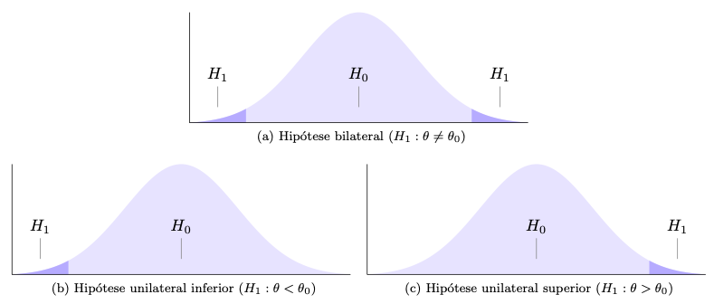
6.3.5 Alternative hypothesis \(H_1\)
The definitions in the table above imply three types of alternative hypothesis, as shown in the following figure. A two-tailed or two-tailed test tests an equilibrium hypothesis, generally used when there is no prior definition of the direction of the hypothesis, such as in case of deciding whether or not a currency should be considered balanced. The lower one-tailed test checks the hypothesis that indicates a reference floor, as in the case of deciding on the minimum effectiveness of a treatment (higher , better). The upper one-tailed test evaluates a hypothesis that indicates a reference ceiling, such as in the case of deciding on an action dependent on a maximum rate mortality rate (lower, better).
6.3.5.1 Procedure to define statistical hypotesis
- Write \[\left\{ \begin{array}{l} H_0: \\ H_1: \end{array} \right. \]
- Parameter.
- Value.
- Alternative hypothesis.
Exercise 6.10 For each item below, indicate the hypotheses being tested.
\(\;\) a. The transport company states that, on average, the interval between successive buses on a given line is 15 minutes. An association of public transport users thinks that punctuality is very important, and wants to test the company’s claim.
\(\;\) b. The shock absorbers of cars that circulate in cities last at least 100 thousand kilometers on average, according to information from some specialized workshops. The owner of a car rental company wants to test this claim.
\(\;\) c. A veterinarian claims to have achieved an average daily gain of at least 3 liters of milk per cow with a new feed composition. A livestock farmer believes that the gain is not that great.
\(\;\) d. Some beer bottles state on their labels that they contain 600mL. Inspection bodies want to assess whether or not a factory should be fined for bottling beers with less quantity than indicated on the label.
\(\;\) e. A casino die seems to be rigged, with the value 1 coming up very frequently.
\(\;\) f. A manufacturer claims that its vaccine prevents at least 80% of cases of a disease. A group of doctors suspect that the vaccine is not that efficient. \(\\\)
6.3.6 Test statistic
Based on the premise that \(H_0\) is true, the value(s) described in this hypothesis are compared with the sample data through a measure called test statistic or pivotal quantity. If the test statistic indicates a small distance between the value(s) of \(H_0\) and the statistic, \(H_0\) is admitted or not rejected; if the distance is large, \(H_0\) is rejected*.
The distances that allow or reject \(H_0\) are evaluated in probabilistic terms, indicated in the graphs of Section 6.3.5 respectively by the light and dark regions. The division of these regions is given by critical values, quantiles of the associated distributions that limit the desired significance (\(\alpha\)) or, equivalently, the confidence (\(1-\alpha\)).
6.3.7 Error types
The classical hypothesis testing procedure is based on type I and type II errors. The significance values are associated with the probability of type I error, or the case in which we make a mistake in rejecting a true \(H_0\) hypothesis. This significance value is arbitrary, that is, it must be defined by the decision maker when stipulating the maximum probability of a type I error. The type II error indicates the case of making a mistake by not rejecting a false \(H_0\) hypothesis.
6.3.8 p-value
It is also possible to consider more precise ways of evaluating probabilistic distances from test statistics than simply indicating ‘above’ or ‘below’ a critical value. According to the classic paradigm, a measure is assigned that varies between 0 and 1, called p-value. This measure has multiple definitions and is still widely discussed in the literature, often being misinterpreted. The following definition is based on (Pereira and Wechsler 1993, 161). Consider an experiment producing data \(x\), an observation of \(X\), to test a simple hypothesis \(H_0\) versus \(H_1\).
Definition 6.4 The p-value is the probability, under \(H_0\), of the event composed by all sample points that favor \(H_1\) (against \(H_0\)) at least as much as \(x\) does.
\(H_0\) is rejected if this degree of evidence is low, lower than a reference value called (level of) significance and represented by \(\alpha\); otherwise, admit or do not reject \(H_0\). Note that a high p-value could indicate ‘\(H_0\) is more credible than \(H_1\)’ OR ‘I don’t have information to decide between \(H_0\) and \(H_1\)’. This is the reason for being careful when declaring ‘\(H_0\) is not rejected’.
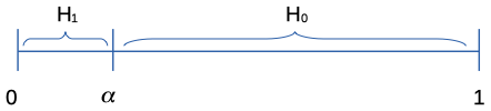
There are typical significance values, usually 10%, 5%, 1%, and 0.1%. Due to an example given by (Ronald A. Fisher 1925)25, the value of 5% became a reference for the value of \(\alpha\), even though there are more elaborate proposals that are better based on Statistical theory. The works of (Pereira and Stern 2020), (Gannon, Pereira, and Polpo 2019) and (Pereira and Wechsler 1993) stand out.
Exercise 6.11 Consider the following image.

by imgflip.com
- Comment on the meme phrase.
- Complete the phrase: ‘If the p is high, …’. \(\\\)
Exercise 6.12 Access https://rpsychologist.com/pvalue/ and carry out the suggested simulations.
6.3.9 Univariate Parametrics
6.3.9.1 TEST UP1 - Single-sample \(t\) test
Hypothesis evaluated
Does a sample of \(n\) subjects (or objects) come from a population mean \(\mu\) equal to a specified value \(\mu_0\)?
Assumptions
A1. The sample was randomly selected from the population it represents.
A2. The distribution of data in the population that the sample represents is normal.
Related tests
TEST 15??? - One-sample Wilcoxon signed-rank test
Test Statistics
Under \(H_0: \mu = \mu_0\),
\[\begin{equation}
t_{test}=\frac{\bar{x}-\mu_0}{s/\sqrt{n}} \sim \mathcal{t}(gl),
\tag{6.8}
\end{equation}\]
where \(gl=n-1\) indicates the degrees of freedom that define the distribution \(t\).
p-value
Under \(H_0: \mu = \mu_0\),
\[\begin{equation}
\text{p-value} = 2Pr(T \le -|t_{test}|).
\tag{6.9}
\end{equation}\]
Under \(H_0: \mu \ge \mu_0\), \[\begin{equation} \text{p-value} = Pr(T \le t_{test}). \tag{6.10} \end{equation}\]
Under \(H_0: \mu \le \mu_0\), \[\begin{equation} \text{p-value} = Pr(T \ge t_{test}). \tag{6.11} \end{equation}\]
Example 6.12 It is desired to test whether the average height of PUCRS students can be considered greater than 167 cm. The test is therefore upper one-tailed in the form \(H_0: \mu \le 167\) vs \(H_1: \mu > 167\). Previous studies indicate that the variable \(X\): ‘height of PUCRS students’ has a normal distribution of unknown mean and standard deviation, indicated by \(X \sim \mathcal{N}(\mu,\sigma)\). From a random sample with \(n=25\) people, \(\bar{x}_{25}=172\) and \(s_{25}=14\) were obtained. Thus, under \(H_0\) the test statistic can be calculated as follows:
\[t_{test} = \frac{172-167}{14/\sqrt{25}} \approx 1.786.\]
If we use \(\alpha=0.05\) (upper one-tailed), \(t_{critical}=1.711\), considering \(gl=24\) degrees of freedom. As the test statistic goes beyond the critical value, i.e., \(1.786 > 1.711\), \(H_0\) is rejected. \(\\\)
Statistical Decision: \(H_0\) is rejected with \(\alpha=5\%\) because \(1.786 > 1.711\).
Experimental Conclusion: The sample suggests that the average height of PUCRS students should be greater than 167 cm.
Example 6.13 In the Example 6.12 it is possible to obtain a range for the p-value associated with the test statistic \(t_{test} \approx 1.786\). As it is an upper one-tailed test, the probability of finding a value as or more extreme than \(t_{test}\) must be obtained according to Equation (6.10). Using the \(t\) table with \(gl=24\) degrees of freedom, \(Pr(t>1.711) = 0.05\) and \(Pr(t>2.064) = 0.025\) are obtained. Given the precision limitation of the \(t\) table, one can only conclude that \(0.025 < Pr(t>1.786) < 0.05\). Using one-tailed \(\alpha=0.05\) we decide again to reject \(H_0\) since the p-value is lower than the significance level, i.e., \(Pr(t>1.786) < 0.05\). The decision made in this way should always be the same when comparing the test statistic with the critical value(s). \(\\\)
Statistical Decision: \(H_0\) is rejected with \(\alpha=5\%\) because \(Pr(t>1.786) < 0.05\).
Experimental Conclusion: The sample suggests that the average height of PUCRS students should be greater than 167 cm.
# Defining the values indicated in the statement
mu0 <- 167
n <- 25
x_bar <- 172
s <- 14
(tt <- (x_bar-mu0)/(s/sqrt(n))) # test statistics, note the greater accuracy
## [1] 1.785714curve(dt(x, df = n-1), -3, 3) # t curve with gl=25-1=24
abline(v = qt(.95, df = n-1), col = 'red') # critical value of ≈1.711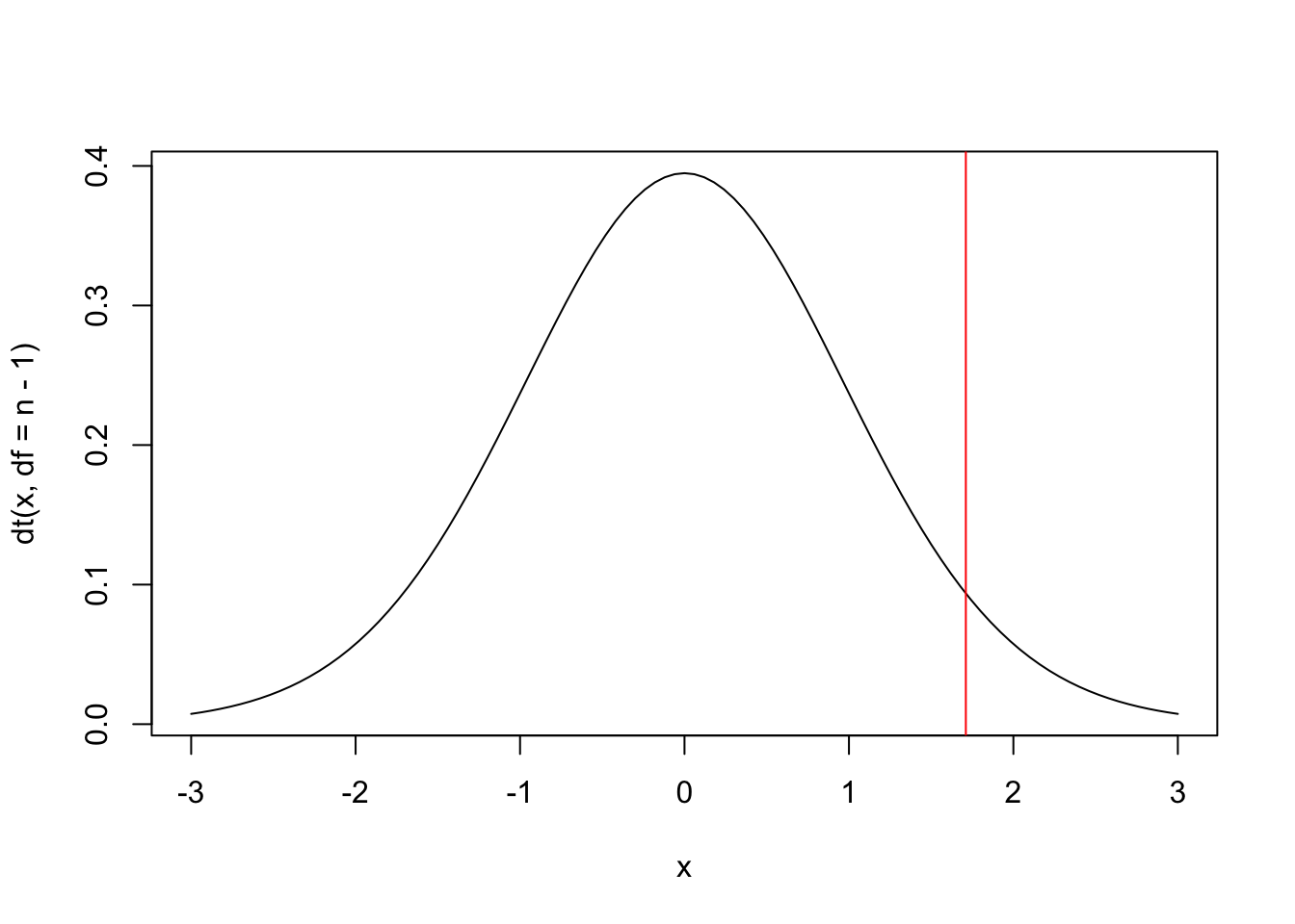
## [1] 0.043394536.3.9.2 TEST UP2 - Tests for one-sample proportion, binomial (exact) and normal (asymptotic)
Hypothesis evaluated
In a population made up of two categories, is the proportion \(\pi\) of observations in one of the categories equal to a specific value \(\pi_0\)?
Assumptions
A1. Each observation can be classified as success or failure.
A2. Each of the \(n\) (conditionally) independent observations is randomly selected from a population.
A3. The probability of success \(\pi\) remains constant for each observation.
Test statistics (asymptotic)
Under \(H_0: \pi = \pi_0\),
\[\begin{equation}
z_{teste}=\frac{p-\pi_0}{\sqrt{\pi_0 (1-\pi_0)/n}} \sim \mathcal{N}(0,1).
\tag{6.12}
\end{equation}\]
p-value (asymptotic)
Under \(H_0: \pi = \pi_0\),
\[\begin{equation}
\text{Valor-p} = 2Pr(Z \le -|z_{teste}|).
\tag{6.13}
\end{equation}\]
Under \(H_0: \pi \ge \pi_0\), \[\begin{equation} \text{Valor-p} = Pr(Z \le z_{teste}). \tag{6.14} \end{equation}\]
Under \(H_0: \pi \le \pi_0\), \[\begin{equation} \text{Valor-p} = Pr(Z \ge z_{teste}). \tag{6.15} \end{equation}\]
p-value (exact)
Let \(X\) be the number of successes in \(n\) Bernoulli trials. Under \(H_0: \pi = \pi_0\) it turns out that \(X \sim \mathcal{B}(n,\pi_0)\), if \(x>\frac{n}{2}\) and \(I = \{ 0,1,\ldots,n-x, x,\ldots,n \}\),
\[\begin{equation}
\text{p-value} = Pr(n-x \ge X \ge x | \pi = \pi_0) = \sum_{i \in I} {n \choose i} \pi_{0}^i (1-\pi_0)^{n-i},
\tag{6.16}
\end{equation}\]
if \(x<\frac{n}{2}\) and \(I = \{ 0,1,\ldots,x, n-x,\ldots,n \}\), \[\begin{equation} \text{p-value} = Pr(x \ge X \ge n-x | \pi = \pi_0) = \sum_{i \in I} {n \choose i} \pi_{0}^i (1-\pi_0)^{n-i}, \tag{6.17} \end{equation}\]
and \(\text{p-value} = 1\) if \(x=\frac{n}{2}\).
Under \(H_0: \pi \le \pi_0\), \[\begin{equation} \text{p-value} = Pr(X \ge x | \pi = \pi_0) = \sum_{i=x}^{n} {n \choose i} \pi_{0}^i (1-\pi_0)^{n-i} \tag{6.18} \end{equation}\]
Under \(H_0: \pi \ge \pi_0\), \[\begin{equation} \text{p-value} = Pr(X \le x | \pi = \pi_0) = \sum_{i=0}^{x} {n \choose i} \pi_{0}^i (1-\pi_0)^{n-i} \tag{6.19} \end{equation}\]
Example 6.15 Suppose you want to test \(\pi\), the proportion of heads on a coin, in the form \(H_0: \pi \le 0.5\) vs \(H_1 : \pi > 0.5\). To do this, the coin is tossed \(n=12\) times, where \(x=9\) heads and \(n-x=12-9=3\) tails are observed. It is known that \(p=\frac{9}{12}=\frac{3}{4}=0.75\). Considering the asymptotic approach, under \(H_0\) \[z_{test}=\frac{0.75-0.5}{\sqrt{0.5 (1-0.5)/12}} \approx 1.73.\] If we use \(\alpha=0.05\) (upper one-tailed), \(z_{cr\acute{\imath}tico}=1.64\). As the test statistic goes beyond the critical value, i.e., \(1.73 > 1.64\), \(H_0\) is rejected. \(\\\)
Statistical Decision: \(H_0\) is rejected with \(\alpha=5\%\) because \(1.73 > 1.64\).
Experimental Conclusion: The sample suggests that the proportion of heads on the coin should be considered greater than 0.5.
Example 6.16 Consider again the data from Example 6.15. By Equation (??) using the standard normal table (with lower precision than the computer), \[\text{p-value} = Pr(Z \ge 1.73) = 1-Pr(Z<1.73) = 1-0.9582 = 0.0418.\] Using one-tailed \(\alpha=0.05\) it is decided again to reject \(H_0\) since the p value is lower than the level of significance, i.e., \(0.0418 < 0.05\). The decision made in this way should always be the same when comparing the test statistic with the critical value(s). \(\\\)
Statistical Decision: \(H_0\) is rejected with \(\alpha=5\%\) because \(0.0418 < 0.05\).
Experimental Conclusion: The sample suggests that the proportion of heads on the coin should be considered greater than 0.5.
## [1] 0.75## [1] 1.732051## [1] 0.04163226# using the prop.test function, without Yates' correction
prop.test(x, n, pi0, alternative = 'greater', correct = FALSE)##
## 1-sample proportions test without continuity correction
##
## data: x out of n, null probability pi0
## X-squared = 3, df = 1, p-value = 0.04163
## alternative hypothesis: true p is greater than 0.5
## 95 percent confidence interval:
## 0.512662 1.000000
## sample estimates:
## p
## 0.75Example 6.18 Consider again the data from Example 6.15. The exact test can be performed considering that under \(H_0: \pi \le 0.5\), the number of heads (successes) \(X\) has binomial distribution of parameters \(n=12\) and \(\pi=0.5\), i.e., \(X \sim \mathcal{B}(12,0.5)\). Thus, the exact p-value results in
\[\begin{equation}
Pr\left( X \geq 9 | \pi = 0.5 \right) = \left[ \binom {12}{9} + \binom {12}{10} + \binom {12}{11} + \binom {12}{12} \right] \times 0.5^{12} \approx 0.0730. \nonumber
\end{equation}\]
Note the difference in the exact value compared to the asymptotic one.
Statistical Decision: \(H_0\) is not rejected with \(\alpha=5\%\) because \(0.0730 > 0.05\).
Experimental Conclusion: the sample suggests that the proportion of heads on the coin can be considered less than or equal to 0.5.
Example 6.19 Performing the Example 6.18 in R.
# manually
n <- 12
x <- 9
pi0 <- 0.5
p9 <- dbinom(9,n,pi0)
p10 <- dbinom(10,n,pi0)
p11 <- dbinom(11,n,pi0)
p12 <- dbinom(12,n,pi0)
p9+p10+p11+p12 # p-value
## [1] 0.07299805##
## Exact binomial test
##
## data: x and n
## number of successes = 9, number of trials = 12, p-value = 0.073
## alternative hypothesis: true probability of success is greater than 0.5
## 95 percent confidence interval:
## 0.4726734 1.0000000
## sample estimates:
## probability of success
## 0.75# using the prop.test function (asymptotic but with Yates continuity correction)
prop.test(x, n, pi0, alternative = 'greater')##
## 1-sample proportions test with continuity correction
##
## data: x out of n, null probability pi0
## X-squared = 2.0833, df = 1, p-value = 0.07446
## alternative hypothesis: true p is greater than 0.5
## 95 percent confidence interval:
## 0.4713103 1.0000000
## sample estimates:
## p
## 0.75References
“The value for which P=.05, or 1 in 20, is 1.96 or nearly 2; it is convenient to take this point as a limit in judging whether a deviation is to be considered significant or not. Deviations exceeding twice the standard deviation are thus formally regarded as significant.” Ronald Aylmer Fisher in the first edition of his book Statistical Methods For Research Workers, from 1925.↩︎