2.2 Frequency Distribution

(Agresti and Franklin 2013, 30) define a frequency distribution as “a listing of possible values for a variable, together with the number of observations at each value”. In this text a distinction will be made between the discrete frequency distribution in Section 2.2.2 and the continuous frequency distribution in Section 2.2.3.

2.2.1 Raw Data, List/Array and Order Statistics

When a variable of interest is observed, in general, the results are recorded in the order in which they appear. This unordered set of data is known as the raw data. When these data are ordered – in ascending or descending order – a list or array is obtained, originating the order statistics. In a distribution of \(n\) elements \(x_{1}\), \(x_{2}\), \(\ldots\), \(x_{n}\) observed sequentially, the data sorted in ascending order is denoted by \(x_{(1)}\), \(x_{(2)}\), \(\ldots\), \(x_{(n)}\) and, similarly, \(x_{(n)}\), \(x_{(n-1)}\) , \(\ldots\), \(x_{(1)}\) for descending sort order.

Example 2.11 (List) If we order the observed data of the variable \(X\): ‘number of steps to the nearest trash can’ from Example 1.6, we obtain the list according to the table below. The lowest number of steps walked was seven, represented by \(x_{(1)}=7\), and the highest was four hundred and two, represented by \(x_{(6)}=402\).

\(x_{(1)}\)	\(x_{(2)}\)	\(x_{(3)}\)	\(x_{(4)}\)	\(x_{(5)}\)	\(x_{(6)}\)
7	20	124	186	191	402

(x <- c(186,402,191,20,7,124))  # Creating and presenting the original raw data vector

## [1] 186 402 191  20   7 124

sort(x)                     # Calculating the list, array or ordered vector. Test ?order

## [1]   7  20 124 186 191 402

sort(x, decreasing = T)     # Descending order, where T indicates TRUE (default: FALSE)

## [1] 402 191 186 124  20   7

At first glance these definitions may seem outdated, but they are of great importance in the construction of advanced data analysis methods. As we currently work with databases in electronic format, it is generally easy to sort large volumes of data. It is important to point out, however, that in certain cases a lot of processing power is needed to perform such sorting, which may have high computational cost. For more details see (Mahmoud 2000) and 15 Sorting Algorithms in 6 Minutes by Timo Bingmann.

Exercise 2.3 Consider the data set \(10,-4,5,7,1,3,9\).

1. Get the list.
2. Indicate and interpret \(x_{(4)}\).

Suggestion: Chapter 8 \(\\\)

Exercise 2.4 Consider the children and height columns available at https://filipezabala.com/data/hospital.csv. Find the list of each one of them using the following functions:

1. base::sort.
   
2. base::order
   
3. dplyr::arrange

Suggestion: Chapter 8 \(\\\)

2.2.2 Discrete frequency distribution

Very long lists, even if ordered, are not usually easy to understand. Thus, the discrete frequency distribution is a good way to consolidate data for a variable that takes, as a rule of thumb, up to 10 different values. This table must have at least one column describing the variable of interest and a column with the frequency (of the class), i.e., the number of observations included in each category. It is also suggested to present a column indicating the class, denoted by \(i\) according to the table below.

\(i\)	\(x_{i}\)	\(f_{i}\)	\(f_{r_{i}}\)	\(F_{i}\)	\(F_{r_{i}}\)	\(\Finv_{i}\)	\(\Finv_{r_{i}}\)
1	\(x_{1}\)	\(f_{1}\)	\(f_{1}/n\)	\(F_{1}=f_{1}\)	\(F_{1}/n\)	\(\Finv_{1}=\Finv_{2}+f_{1}=n\)	\(\Finv_{1}/n=1\)
2	\(x_{2}\)	\(f_{2}\)	\(f_{2}/n\)	\(F_{2}=F_{1}+f_{2}\)	\(F_{2}/n\)	\(\Finv_{2}=\Finv_{3}+f_{2}\)	\(\Finv_{2}/n\)
3	\(x_{3}\)	\(f_{3}\)	\(f_{3}/n\)	\(F_{3}=F_{2}+f_{3}\)	\(F_{3}/n\)	\(\Finv_{3}=\Finv_{4}+f_{3}\)	\(\Finv_{3}/n\)
\(\vdots\)	\(\vdots\)	\(\vdots\)	\(\vdots\)	\(\vdots\)	\(\vdots\)	\(\vdots\)	\(\vdots\)
\(k-2\)	\(x_{k-2}\)	\(f_{k-2}\)	\(f_{k-2}/n\)	\(F_{k-2}=F_{k-3}+f_{k-2}\)	\(F_{k-2}/n\)	\(\Finv_{k-2}=\Finv_{k-1}+f_{k-2}\)	\(\Finv_{k-2}/n\)
\(k-1\)	\(x_{k-1}\)	\(f_{k-1}\)	\(f_{k-1}/n\)	\(F_{k-1}=F_{k-2}+f_{k-1}\)	\(F_{k-1}/n\)	\(\Finv_{k-1}=\Finv_{k}+f_{k-1}\)	\(\Finv_{k-1}/n\)
\(k\)	\(x_{k}\)	\(f_{k}\)	\(f_{k}/n\)	\(F_{k}=F_{k-1}+f_{k}=n\)	\(F_{k}/n=1\)	\(\Finv_{k}=f_{k}\)	\(\Finv_{k}/n\)
Total	-	\(n\)	1	-	-	-	-

For the generic class \(i\) the following frequencies are calculated:
- \(f_{i}\): Frequency
- \(f_{r_{i}}\): Relative frequency
- \(F_{i}\): Cumulative frequency
- \(F_{r_{i}}\): Cumulative relative frequency
- \(\Finv_{i}\): Inverse cumulative frequency
- \(\Finv_{r_{i}}\): Relative inverse cumulative frequency

Example 2.12 (Number of children revisited) From the Example 2.4 the following variable was observed:

\(X\): ‘number of children of women assisted in a hospital’.

The following table of raw data shows the data in the order in which it was observed. This type of presentation is quite complete, but makes it difficult to extract relevant information. As an exercise, indicate the maximum number of children observed in the sample from this table.

\(i\)	\(x_{i}\)	\(i\)	\(x_{i}\)	\(i\)	\(x_{i}\)	\(i\)	\(x_{i}\)	\(i\)	\(x_{i}\)
1	2	21	2	41	1	61	3	81	0
2	0	22	3	42	1	62	0	82	1
3	1	23	1	43	4	63	2	83	2
4	2	24	2	44	1	64	0	84	2
5	4	25	2	45	1	65	2	85	2
6	2	26	1	46	3	66	2	86	2
7	1	27	4	47	1	67	2	87	2
8	4	28	0	48	1	68	1	88	4
9	2	29	1	49	4	69	2	89	0
10	3	30	6	50	2	70	3	90	2
11	3	31	1	51	2	71	1	91	1
12	2	32	1	52	4	72	3	92	3
13	3	33	1	53	1	73	1	93	3
14	2	34	1	54	3	74	3	94	4
15	1	35	0	55	1	75	3	95	5
16	4	36	2	56	2	76	4	96	1
17	2	37	3	57	0	77	2	97	0
18	0	38	3	58	2	78	1	98	0
19	1	39	1	59	3	79	2	99	3
20	4	40	2	60	3	80	3	100	2

The following table presents the frequency distribution of the number of children. With the presentation in this format, the maximum of 6 children is easily observed in the sample, unlike the raw data table. Only the order in which the data were observed is lost, which is generally not in the interest of the researcher.

\(i\)	\(x_{i}\)	\(f_{i}\)	\(f_{r_{i}}\)	\(F_{i}\)	\(F_{r_{i}}\)	\(\Finv_{i}\)	\(\Finv_{r_{i}}\)
1	0	11	\(11/100=0.11\)	11	\(11/100=0.11\)	\(89+11=100\)	\(100/100=1\)
2	1	27	\(27/100=0.27\)	\(11+27=38\)	\(38/100=0.38\)	\(62+27=89\)	\(89/100=0.89\)
3	2	30	\(30/100=0.30\)	\(38+30=68\)	\(68/100=0.68\)	\(32+30=62\)	\(62/100=0.62\)
4	3	19	\(19/100=0.19\)	\(68+19=87\)	\(87/100=0.87\)	\(13+19=32\)	\(32/100=0.32\)
5	4	11	\(11/100=0.11\)	\(87+11=98\)	\(98/100=0.98\)	\(2+11=13\)	\(13/100=0.13\)
6	5	1	\(1/100=0.01\)	\(98+1=99\)	\(99/100=0.99\)	\(1+1=2\)	\(2/100=0.02\)
7	6	1	\(1/100=0.01\)	\(99+1=100\)	\(100/100=1\)	1	\(1/100=0.01\)
Total	-	100	1	-	-	-	-

Note that the column \(i\) in the raw data table indicates the order of the woman interviewed, while in the frequency distribution \(i\) indicates the class. For example, \(i=4\) indicates the fourth woman interviewed, who in this case reported having \(x_{4}=2\) children. In the frequency distribution, \(i=4\) indicates the fourth class where \(x_{4}=3\), i.e., the class of women who have 3 children.

The only columns that require reading the raw data are the variable \(x_i\) and the frequency \(f_i\); the others are calculated from \(f_i\). Below are some examples of interpreting the frequencies shown in the frequency distribution.
- \(f_{5}=11\), i.e., 11 women have 4 children
- \(f_{r_{5}}=0.11=11\%\), i.e., 11% of women have 4 children
- \(F_{4}=87\), i.e., 87 women have up to 3 children (or ‘from zero to 3 children’, but this is less elegant)
- \(F_{r_{3}}=0.68=68\%\), i.e., 68% of women have up to 2 children
- \(\Finv_{3}=62\), i.e., 62 women have at least 2 children
- \(\Finv_{r_{2}}=0.89=89\%\), i.e., 89% of women have at least 1 child

Example 2.13 (Number of children R-visited) Example 2.12 using R/RStudio.

h <- read.csv('https://filipezabala.com/data/hospital.csv')
dim(h)       # Dimension: 100 rows by 2 columns

## [1] 100   2

n <- nrow(h) # Number of rows of h
head(h)      # Displays the first 6 rows of the 'h' object; test tail(h, 10)

##   children height
## 1        2   1.59
## 2        0   1.58
## 3        1   1.70
## 4        2   1.62
## 5        4   1.67
## 6        2   1.62

(tab <- table(h$children))    # Frequency

## 
##  0  1  2  3  4  5  6 
## 11 27 30 19 11  1  1

prop.table(tab)               # Relative frequency

## 
##    0    1    2    3    4    5    6 
## 0.11 0.27 0.30 0.19 0.11 0.01 0.01

cumsum(tab)                   # Cumulative frequency

##   0   1   2   3   4   5   6 
##  11  38  68  87  98  99 100

round(cumsum(tab)/n,2)        # Cumulative relative frequency

##    0    1    2    3    4    5    6 
## 0.11 0.38 0.68 0.87 0.98 0.99 1.00

cumsum(rev(tab))              # Inverse cumulative frequency

##   6   5   4   3   2   1   0 
##   1   2  13  32  62  89 100

round(cumsum(rev(tab))/n,2)   # Relative inverse cumulative frequency

##    6    5    4    3    2    1    0 
## 0.01 0.02 0.13 0.32 0.62 0.89 1.00

Exercise 2.5 In a factory, a sample of 50 pieces was taken from a batch of certain material and the number of defects in each piece was counted, shown in the table below.

\(i\)	# defects	\(f_i\)	\(fr_i\)	\(F_i\)	\(Fr_i\)	\(\Finv_{i}\)	\(\Finv_{r_{i}}\)
1	0	17
2	1	10
3	2
4	3	8
5	4	5
6	5	1
Total	-	50

1. Classify the variable ‘number of defects’.
   
2. What is the frequency of class 3? Interpret the value.
   
3. What is the relative frequency of class 3? Interpret the value.
   
4. What is the cumulative frequency of class 4? Interpret the value.
   
5. What is the cumulative relative frequency of class 5? Interpret the value.

Suggestion: Chapter 8

2.2.3 Continuous frequency distribution

As a rule of thumb, when a variable assumes more than 10 different values it is recommended to use the continuous frequency distribution. The difference to the discrete distribution of Section 2.2.2 is that in the continuous one the values are distributed in class intervals, i.e., ranges of values with a certain amplitude. The main advantage of this approach is the ability to present the data in a lean way. The counterpoint, as with any data summary, is the loss of the original information.

Class interval and number of classes

Below are three of the main rules for determining the class interval (\(C\)) and the number of classes (\(k\)) of a statistical series with \(n\) items.

1. Sturges

This formula (…) is based on the principle that the proper distribution into classes is given, for all numbers which are powers of 2, by a series of binomial coefficients. For example, 16 items would be divided normally into 5 classes, with class frequencies 1, 4, 6, 4, 1. (Sturges 1926, 65)

Based on the aforementioned principle, (Sturges 1926) suggests that the class interval be calculated by \[\begin{equation} C_{St} = \frac{R}{k_{St}} = \frac{\max{X}-\min{X}}{1 + \log_{2}{n}} \approx \frac{\max{X}-\min{X}}{1 + 3.322 \log_{10}{n}}, \tag{2.1} \end{equation}\]

where \(R\) is the range described in Section 2.4.1. The denominator is obtained from the binomial expansion, in the form \[\begin{equation} n = \sum_{i=0}^{k-1} {k-1 \choose i} = (1+1)^{k-1} = 2^{k-1}. \tag{2.2} \end{equation}\]

From the Equation (2.2) one can get

\[\begin{equation} k_{St} = \left\lceil 1 + \log_{2}{n} \right\rceil \approx \left\lceil 1 + 3.322 \log_{10}{n} \right\rceil, \tag{2.3} \end{equation}\]

where \(\left\lceil \;\; \right\rceil\) indicates the ceiling function according to Eq. (1.4). Some computational packages assign the number of classes by applying rules that find a ‘pretty’ value for the division.

The most convenient class intervals are 1, 2, 5, 10, 20, etc., so that in practice the formula for the theoretical class interval may be used as a means of choosing among these convenient ones. In general the next smaller convenient class interval should be chosen, that is, the one next below the theoretically optimal interval. If the formula gives 9, 10 may be chosen, but if the formula indicates 7 or 8, the one actually used should generally be the next lower convenient class interval 5. (Sturges 1926, 65)

Example 2.14 If \(n=100\) values with amplitude \(R=0.23\) are observed, the class interval suggested by Sturges is \[C_{St} = \frac{0.23}{1 + \log_{2}{100}} = 0.02875,\] and the number of classes \[k_{St} = \left\lceil 1 + \log_{2}{100} \right\rceil = \left\lceil 7.644 \right\rceil = 8.\]

n <- length(h$height)             # n=100, number of data to be tabulated
R <- diff(range(h$height))        # Range
ceiling(1 + log2(n))              # By Equation (2.3), using log2

## [1] 8

ceiling(1 + 3.322*log10(n))       # By Equation (2.3), usando log10

## [1] 8

(kSt <- nclass.Sturges(h$height)) # k obtained by the function 'nclass.Sturges'

## [1] 8

(CSt <- R/kSt)                    # By Equation (2.1)

## [1] 0.02875

pretty(kSt)                       # Pretty breakpoints

## [1]  5 10

2. Scott

(Scott 1979) incorporates \(s\), the sample standard deviation according to Eq. (2.27), into the calculation of the class interval. \[\begin{equation} C_{Sc} = \dfrac{3.49\,s}{\sqrt[3]{n}}. \tag{2.4} \end{equation}\]

The number of Scott classes can be obtained by \[\begin{equation} k_{Sc} = \left\lceil \dfrac{R}{C_{Sc}} \right\rceil = \left\lceil \dfrac{\max{X} - \min{X}}{3.49\,s/\sqrt[3]{n}} \right\rceil. \tag{2.5} \end{equation}\]

Example 2.15 (Scott) If \(n=100\) values with sample standard deviation \(s=0.045268559\) are observed, the class interval suggested by Scott is \[C_{Sc} = \dfrac{3.49 \times 0.045268559}{100^{1/3} } \approx 0.03403732562.\] If \(R=0.23\), the number of classes is \[k_{Sc} =\left\lceil \dfrac{0.23}{0.03403732562} \right\rceil = \left\lceil 6.757288 \right\rceil = 7.\]

n <- length(h$height)             # n=100, number of data to be tabulated
R <- diff(range(h$height))        # Range
s <- sd(h$height)                 # s=0.045268559, sample standard deviation
(CSc <- 3.49*s/n^(1/3))           # By Eq. (2.4)

## [1] 0.03403732562

ceiling(R/CSc)                    # k suggested by Scott, Eq. (2.5)

## [1] 7

(kSc <- nclass.scott(h$height))   # k obtained by the function 'nclass.scott'

## [1] 7

pretty(kSc)                       # Pretty breakpoints

## [1]  5 10

3. Freedman-Diaconis

Rule: Choose the cell width as twice the interquartile range of the data, divided by the cube root of the sample size. (Freedman and Diaconis 1981, 454)

(Freedman and Diaconis 1981) insert \(IQR\), the interquartile range according Eq. (2.28), into the class interval calculation. \[\begin{equation} C_{FD} = \frac{2\,IQR}{\sqrt[3]{n}}, \tag{2.6} \end{equation}\]

The number of classes obtained as a consequence of applying the Freedman-Diaconis relation is \[\begin{equation} k_{FD} = \left\lceil \frac{R}{C_{FD}} \right\rceil = \left\lceil \frac{\max{X} - \min{X}}{2\,IQR/\sqrt[3]{n}} \right\rceil. \tag{2.7} \end{equation}\]

Example 2.16 (Freedman-Diaconis) If \(n=100\) values with an interquartile range of \(IQR=0.0525\) are observed, the class interval suggested by Freedman-Diaconis is \[C_{FD} = \frac{2 \times 0.0525}{\sqrt[3]{100}} \approx 0.02262156425.\] If \(R=0.23\), the number of classes is \[k_{FD} = \left\lceil \frac{0.23}{0.02262156425} \right\rceil = \left\lceil 10.16729 \right\rceil = 11.\]

n <- length(h$height)                   # n=100, number of data to be tabulated
R <- diff(range(h$height))              # Range
(Q <- quantile(h$height, c(1/4,3/4)))   # First and third quartiles

##    25%    75% 
## 1.5975 1.6500

(IQR <- diff(as.numeric(Q)))    # Interquartile Range

## [1] 0.0525

(CFD <- 2*IQR/n^(1/3))           # By Eq. (2.6)

## [1] 0.02262156425

ceiling(R/CFD)                  # k suggested by Freedman-Diaconis, Eq. (2.7)

## [1] 11

(kFD <- nclass.FD(h$height))    # k obtained by the function 'nclass.FD'

## [1] 11

pretty(kFD)                     # Pretty breakpoints

## [1] 10 20

(Hyndman 1995) argues that the Scott and Freedman-Diaconis rules are as simple as the Sturges rule, but better grounded in statistical theory. Also, Sturges’ rule works well for moderate sample sizes (\(n < 200\)), but not for large values of \(n\).

Example 2.17 (Comparing the three methods) A simulation was performed with sample sizes \(n=10^{i}\), \(i \in \{1, 2, \ldots, 6 \}\), indicating the number of classes suggested by each method.

NC <- function(x) c(i = i, n = 10^i,                 # Simulated quantities
                    Sturges = nclass.Sturges(x),     # Sturges (1926)
                    Scott = nclass.scott(x),         # Scott (1979)
                    FD = nclass.FD(x))               # Freedman-Diaconis (1981)
for(i in 1:6){set.seed(i); print(NC(rnorm(10^i)))}   # May be time consuming for i>6

##       i       n Sturges   Scott      FD 
##       1      10       5       2       3 
##       i       n Sturges   Scott      FD 
##       2     100       8       6       7 
##       i       n Sturges   Scott      FD 
##       3    1000      11      19      25 
##       i       n Sturges   Scott      FD 
##       4   10000      15      44      56 
##       i       n Sturges   Scott      FD 
##       5  100000      18     112     145 
##       i       n Sturges   Scott      FD 
##       6 1000000      21     278     360

Example 2.18 (Women’s heights) Let be the variable

\(Y\): ‘height of women assisted in a hospital’.

The table below presents the raw data. This type of presentation is quite complete, but makes it difficult to extract relevant information. As an exercise, indicate how many women are between 1.70m and 1.75m tall from this table.

\(i\)	\(y_{i}\)	\(i\)	\(y_{i}\)	\(i\)	\(y_{i}\)	\(i\)	\(y_{i}\)
1	1.59	26	1.61	51	1.64	76	1.62
2	1.58	27	1.61	52	1.57	77	1.54
3	1.70	28	1.60	53	1.65	78	1.64
4	1.62	29	1.61	54	1.69	79	1.66
5	1.67	30	1.64	55	1.65	80	1.56
6	1.62	31	1.59	56	1.62	81	1.64
7	1.69	32	1.60	57	1.68	82	1.60
8	1.60	33	1.62	58	1.60	83	1.68
9	1.61	34	1.53	59	1.68	84	1.65
10	1.58	35	1.58	60	1.59	85	1.65
11	1.64	36	1.60	61	1.70	86	1.64
12	1.72	37	1.61	62	1.65	87	1.55
13	1.74	38	1.67	63	1.51	88	1.66
14	1.63	39	1.68	64	1.66	89	1.59
15	1.64	40	1.56	65	1.52	90	1.66
16	1.63	41	1.58	66	1.60	91	1.69
17	1.59	42	1.66	67	1.62	92	1.61
18	1.64	43	1.59	68	1.68	93	1.58
19	1.59	44	1.67	69	1.65	94	1.73
20	1.65	45	1.62	70	1.61	95	1.56
21	1.63	46	1.55	71	1.56	96	1.59
22	1.64	47	1.64	72	1.65	97	1.65
23	1.64	48	1.62	73	1.62	98	1.63
24	1.62	49	1.65	74	1.63	99	1.70
25	1.66	50	1.66	75	1.57	100	1.60

To put these values in a frequency table, \(k_{St}=8\) was obtained by Sturges’ rule, and by the result of pretty(8) we decided on 5 classes.

The table below presents the heights grouped into five classes of 5 cm amplitude, also providing some frequencies that help understanding the distribution. Easily observe 6 women with height between 1.70m and 1.75m,¹¹ contrary to the raw data table. Note, however, that it is not possible to know the exact height of each of these 6 women. This happens because summarizing implies loss of information, and it is up to the researcher to decide when and how to summarize the data.

\(i\)	\(y_{i}\)	\(f_{i}\)	\(f_{r_{i}}\)	\(F_{i}\)	\(F_{r_{i}}\)	\(\Finv_{i}\)	\(\Finv_{r_{i}}\)
1	1.50 \(\vdash\) 1.55	4	0.04	4	0.04	\(96+4=100\)	\(100/100=1\)
2	1.55 \(\vdash\) 1.60	21	0.21	\(4+21=25\)	0.25	\(75+21=96\)	\(96/100=0.96\)
3	1.60 \(\vdash\) 1.65	41	0.41	\(25+41=66\)	0.66	\(34+41=75\)	\(75/100=0.75\)
4	1.65 \(\vdash\) 1.70	28	0.28	\(66+28=94\)	0.94	\(6+28=34\)	\(34/100=0.34\)
5	1.70 \(\vdash\) 1.75	6	0.06	\(94+6=100\)	1	6	\(6/100=0.06\)
Total	-	100	1	-	-	-	-

Below are some examples of interpretation of the frequencies presented in the table above.
- \(f_{5}=6\), i.e., 6 women are between 1.70m and 1.75m tall
- \(f_{r_{5}}=0.06=6\%\), i.e., 6% of women are between 1.70m and 1.75m tall
- \(F_{4}=94\), i.e., 94 women are up to 1.70m tall, or from 1.50m to 1.70m
- \(F_{r_{2}}=0.25=25\%\), i.e., 25% of women are up to 1.60m tall, or from 1.50m to 1.60m
- \(\Finv_{3}=75\), i.e., 75 women are at least 1.60 m tall
- \(\Finv_{r_{4}}=0.34=34\%\), i.e., 34% of women are at least 1.65m tall

\(\\\)

Exercise 2.6 Considering the data from Example ??, get \(k_{Sc}\) and \(k_{FD}\).

Example 2.19 (Heights of women R-visited) Example 2.18 using R/RStudio.

h <- read.csv('https://filipezabala.com/data/hospital.csv')
dim(h)        # Dimension: 100 rows by 2 columns

## [1] 100   2

n <- nrow(h)  # Number of rows
head(h)       # Displays the first 6 lines of object 'h'; test tail(h, 10)

##   children height
## 1        2   1.59
## 2        0   1.58
## 3        1   1.70
## 4        2   1.62
## 5        4   1.67
## 6        2   1.62

pretty(nclass.Sturges(h$height))    # Pretty breakpoints

## [1]  5 10

hi <- hist(h$height, right = FALSE) # Histogram, note right = FALSE

hi$breaks                           # Breaks values generated with the 'hist' function

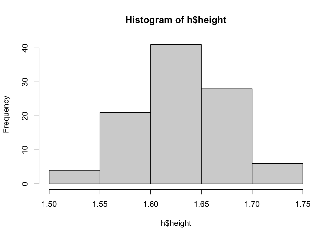
## [1] 1.50 1.55 1.60 1.65 1.70 1.75

(f <- hi$counts)                    # Class frequencies

## [1]  4 21 41 28  6

cumsum(f)                           # Cumulative frequency

## [1]   4  25  66  94 100

round(cumsum(f)/n, 2)       # Relative cumulative frequency

## [1] 0.04 0.25 0.66 0.94 1.00

cumsum(rev(f))              # Inverse cumulative frequency

## [1]   6  34  75  96 100

round(cumsum(rev(f))/n, 2)  # Relative inverse cumulative frequency

## [1] 0.06 0.34 0.75 0.96 1.00

Exercise 2.7 Considering the Example 2.19, indicate:

a.What happens when you use right = FALSE? What’s the difference to right = TRUE?
b. What algorithm is being used in calculating h$breaks? How is it possible to change this presentation?

\(\\\)

References

Agresti, Alan, and Christine A Franklin. 2013. Statistics: The Art and Science of Learning from Data. Pearson Education MUA. https://toc.library.ethz.ch/objects/pdf_ead50/5/E50_010307250_TB-Inhalt_005862608.pdf.

Freedman, David, and Persi Diaconis. 1981. “On the Histogram as a Density Estimator: L2 Theory.” Zeitschrift für Wahrscheinlichkeitstheorie Und Verwandte Gebiete 57 (4): 453–76. https://link.springer.com/content/pdf/10.1007/BF01025868.pdf.

Hyndman, Rob J. 1995. “The Problem with Sturges Rule for Constructing Histograms.” http://robjhyndman.com/papers/sturges.pdf.

Mahmoud, Hosam M. 2000. Sorting: A Distribution Theory. Vol. 54. John Wiley & Sons.

Scott, David W. 1979. “On Optimal and Data-Based Histograms.” Biometrika 66 (3): 605–10. http://materias.df.uba.ar/mtb2019c1/files/2014/08/On-optimal-and-Data-based-histograms.pdf.

Sturges, Herbert A. 1926. “The Choice of a Class Interval.” Journal of the American Statistical Association 21 (153): 65–66. http://www.esalq.usp.br/departamentos/lce/arquivos/aulas/2013/LCE0216/Sturges1926.pdf.

---

11. Note that the symbology 1.70 \(\vdash\) 1.75 indicates the inclusion of 1.70 and the exclusion of 1.75, i.e., this is an interval closed on the left and open on the right. Equivalent to the notations \(\left[ 1.70, 1.75 \right[\) (more modern) or \(\left[ 1.70, 1.75 \right)\) (older).↩︎