3.7 Special Discrete Distributions
For more details it is recommended (Johnson, Kemp, and Kotz 2005). McLaughlin (2016) brings a compendium of probability distributions.
3.7.1 Discrete uniform \(\cdot \; \mathcal{DU}(a,b)\)
\[\begin{equation} p(x|a,b) = \frac{1}{b-a+1} \tag{3.48} \end{equation}\]
where \(a\) and \(b\) are integers such that \(b \ge a\).
3.7.2 Binomial \(\cdot \; \mathcal{B}(n,p)\)
Consider a single toss of a coin that results in heads (\(H\)) or tails (\(T\)). Let \(Pr(\{ H \})=p\) and \(Pr(\{ T \})=1-p\). This is a Bernoulli trial. Now suppose \(n\) independent flips of the same coin, and let \(X\) be the number of heads resulting in the \(n\) independent tosses. \(X\) is a random variable (with probability) binomial distribution of parameters \(n\) and \(p\), denoted by \(X \sim \mathcal{B}(n,p)\). The probability mass function is
\[\begin{equation} p(x|n,p) = Pr(X=x) = {n \choose x}p^{x}(1-p)^{n-x} \tag{3.49} \end{equation}\]
where \(n \in \mathbb{N}, p \in \left[ 0,1 \right]\), \(x \in \left\lbrace 0, \ldots, n \right\rbrace\) and \({n \choose x}\) is defined by Eq. (3.19).
The expected value and variance are given by
\[\begin{equation} E(X)=np \tag{3.50} \end{equation}\]
\[\begin{equation} V(X)=np(1-p) \tag{3.51} \end{equation}\]
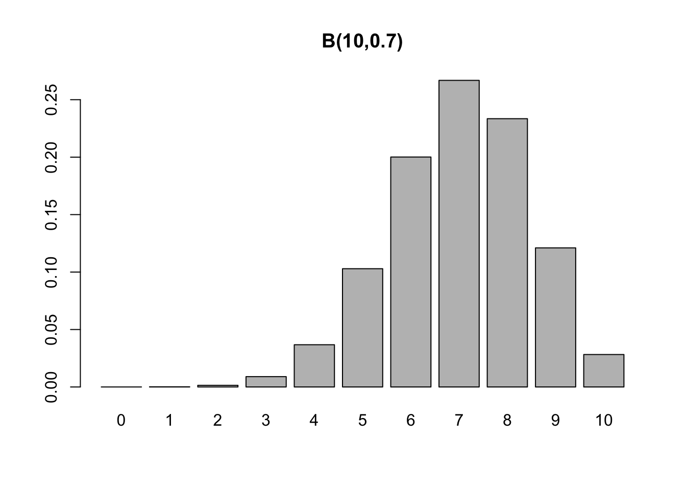
Example 3.26 (Binomial) Suppose \(n=10\) flips of a coin with \(p=0.7\). Thus, \[ X \sim \mathcal{B}(10,0.7),\] \[ p(x) = Pr(X=x) = {10 \choose x} 0.7^{x} 0.3^{10-x}, \] \[ E(X)=10 \times 0.7 = 7, \] \[ V(X)=10 \times 0.7 \times 0.3 = 2.1. \] %\[ D(X) = \sqrt{2.1} \approx 1.449138. \]
3.7.3 Negative Binomial \(\cdot \; \mathcal{BN}(k,p)\)
Consider again the flip of a coin that results in heads (\(H\), success) or tails (\(T\), failure) where \(Pr(\{ H \})=p\) and \(Pr(\{ T \}) =1-p\). Let \(X\) be the ‘number of failures until the \(s\)-th success’. \(X\) is a random variable with negative binomial distribution of parameters \(s\) and \(p\), denoted by \(X \sim \mathcal{BN}(s,p)\), defined by
\[\begin{equation} p(x|k,p) = Pr(X=x) = {x+s-1 \choose x}p^{s}(1-p)^{x} \tag{3.52} \end{equation}\]
where \[ k \in \{1,2,\ldots\}, 0 \le p \le 1, x \in \{0,1,\ldots\} \] and
\[\begin{equation} {x+k-1 \choose x} = C_{x}^{x+k-1} = \frac{{(x+k-1)!}}{{x!(k-1)!}} \tag{3.53} \end{equation}\]
The expected value and variance are given by
\[\begin{equation} E(X)=\frac{pk}{1-p} \tag{3.54} \end{equation}\]
\[\begin{equation} V(X)=\frac{pk}{(1-p)^2} \tag{3.55} \end{equation}\]
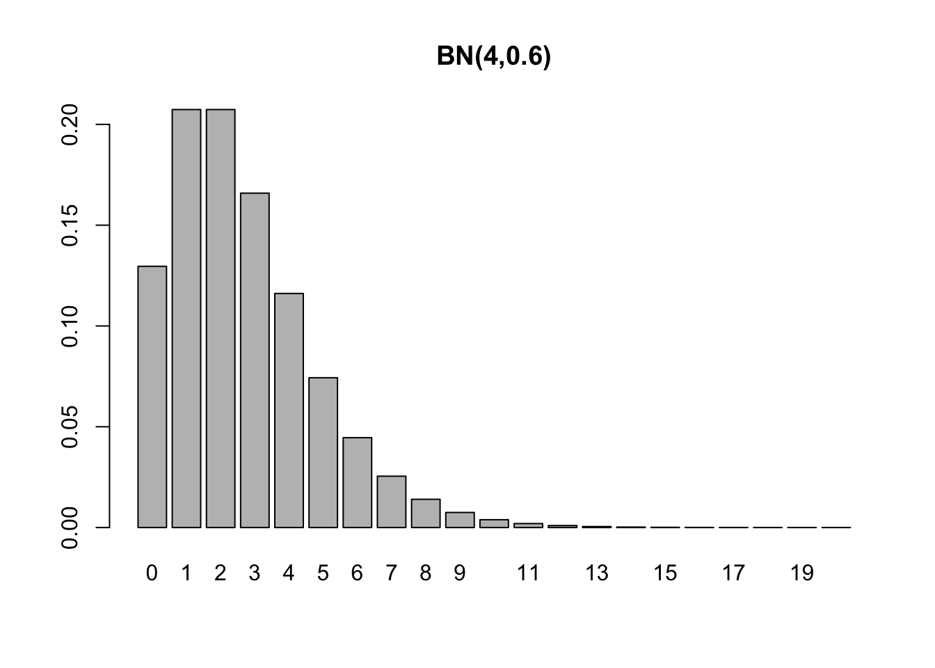
Example 3.27 (Negative binomial) A coin with \(p=0.6\) is tossed until \(k=4\) heads are obtained. \[ X \sim \mathcal{BN}(4,0.6),\] \[ p(x) = Pr(X=x) = {x+3 \choose x} 0.6^{4} 0.4^{x}, \] \[ E(X) = \frac{0.6 \times 4}{1-0.6} = 6 \] \[ V(X)= \frac{0.6 \times 4}{(1-0.6)^2} = 15 \] \[ D(X) = \sqrt{15} \approx 3.873. \]
The functions dnbinom and its corresponding functions (pbinom, qbinom and rbinom) model the variable \(X\) according to Eq. (3.52). For alternative formulations see this Wikipedia article.
bn <- function(x,k,p){
  choose(x+k-1,x) * p^k * (1-p)^x
}
all.equal(bn(0:20, 4, 0.6), dnbinom(0:20, 4, 0.6))
## [1] TRUE3.7.4 Poisson \(\cdot \; \mathcal{P}(\lambda)\)
Siméon Denis Poisson approached the distribution that bears his name considering the limit of a sequence of binomial distributions according to Equation (3.49), in which \(n\) tends to infinity and \(p\) tends to zero while \(np\) remains finitely equal to \(\lambda\) (Poisson 1837). The term ‘Poisson distribution’ (Poisson-Verteilung) was coined by (Bortkewitsch 1898), although Abraham de Moivre derived this distribution more than a century before (De Moivre 1718), (De Moivre 1756), (Stigler 1982).
Example 3.28 Consider a tollbooth where on average \(\lambda\) vehicles pass per minute. The discrete r.v. \(X\): ‘number of vehicles per minute’ has Poisson distribution of parameter \(\lambda\), denoted by \(X \sim \mathcal{P}(\lambda)\), where \(x \in \left \lbrace 0, 1, 2, \ldots \right\rbrace\) and \(\lambda > 0\).
The probability mass function is given by
\[\begin{equation} p(x|\lambda) = Pr(X=x) = \frac{{e^{ - \lambda } \lambda ^x }}{{x!}} \tag{3.56} \end{equation}\]
where the Euler’s number19 has an approximate value \(e \approx 2.71828\;18284\;59045\;23536\). The expected value and variance are given by
\[\begin{equation}
E(X)=\lambda
\tag{3.57}
\end{equation}\]
\[\begin{equation} V(X)=\lambda \tag{3.58} \end{equation}\]
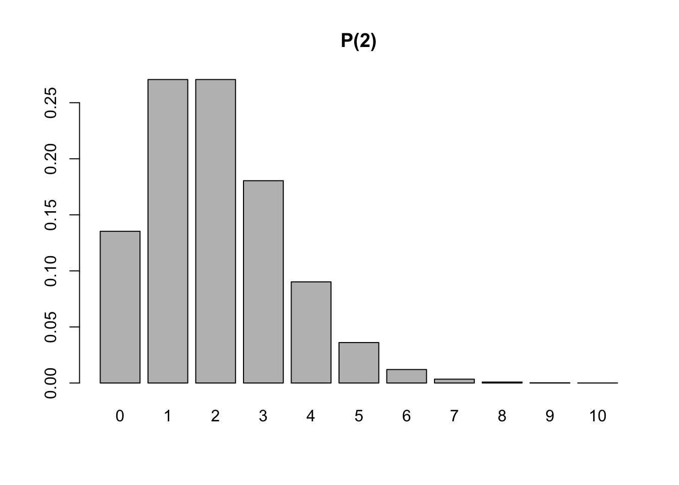
Example 3.29 (Poisson) Consider a tollbooth where an average of \(\lambda = 2\) vehicles pass per minute. Thus, \[ X \sim \mathcal{P}(2),\] \[ p(x) = Pr(X=x) = \frac{{e^{- 2} 2^{x} }}{{x!}}, \] \[ E(X)=2, \] \[ V(X)=2. \] \[ D(X) = \sqrt{2} \approx 1.4142. \]
Exercise 3.16 Consider the Poisson distribution and the exponential function defined by the series \(\sum_{x=0}^{\infty} \frac{\lambda^x}{x!} = e^\lambda\) (Boros and Moll 2004, 91). a. Show that the function described by Eq. (3.56) is a probability (mass) function. b. Show that \(E(X)\) is given by Eq. (3.57). c. Show that \(V(X)\) is given by Eq. (3.58).
Solution: Chapter 8 \(\\\)
3.7.5 Hypergeometric \(\cdot \; \mathcal{H}(N,R,n)\)
Suppose an urn with \(N\) balls of which \(R\) are marked with a \(\times\), from which a sample of \(n\) balls is taken. Let \(X\) be the number of marbles marked with \(\times\) of the \(n\) drawn. \(X\) has hypergeometric distribution, denoted by \[ X \sim \mathcal{H}(N,R,n) \] where \(x \in \left\lbrace 0, 1, \ldots, n \right\rbrace\), \(N \in \{1,2,\ldots\}\), \(R \in \{1,2,\ldots,N\}\), \(n \in \{1,2,\ldots ,N\}\)}. Its probability mass function is defined by
\[\begin{equation} p(x|N,R,n) = Pr(X=x) = \dfrac{{R \choose x}{N-R \choose n-x}}{{N \choose n}} \tag{3.59} \end{equation}\]
The expected value and variance are given by
\[\begin{equation}
E(X) = n \frac{R}{N}
\tag{3.60}
\end{equation}\]
\[\begin{equation} V(X) = n \frac{R}{N} \frac{N-R}{N} \frac{N-n}{N-1} \tag{3.61} \end{equation}\]
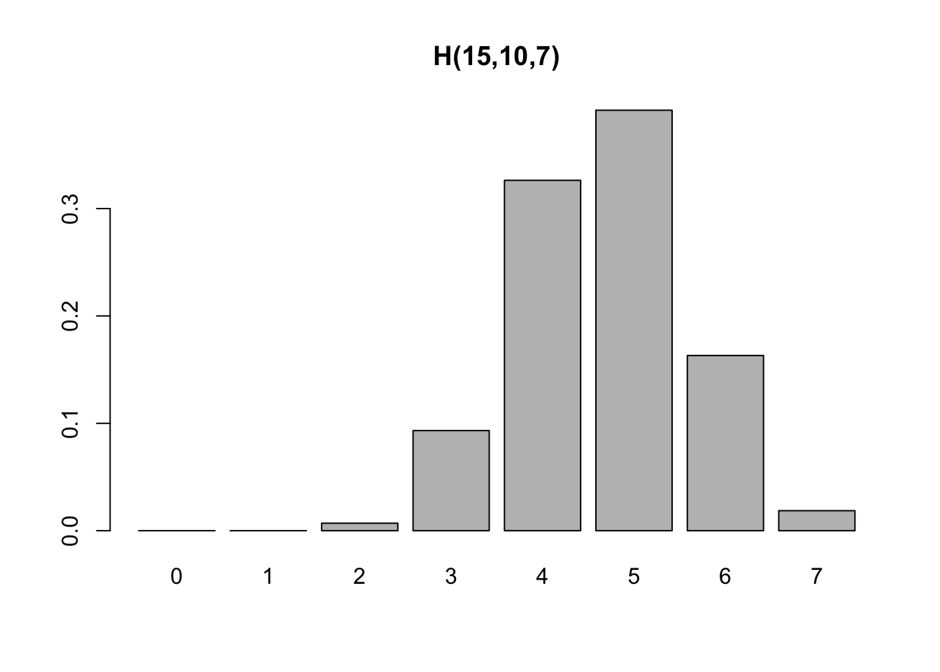
Example 3.30 (Hypergeometric) Suppose an urn with \(N=15\) balls, \(R=10\) marked with a \(\times\) from which a sample of \(n=7\) balls is taken.
3.7.6 Bernoulli-Poisson \(\cdot \; \mathcal{BP}(p,\lambda_1,\lambda_2)\)
A random variable \(X\) has a Bernoulli-Poisson distribution parameterized by \(p\), \(\lambda_1\) and \(\lambda_2\) if it assumes a Poisson distribution of rate \(\lambda_1\) with probability \(p\) and a Poisson distribution of rate \(\ lambda_2\) with probability \(1-p\). Symbolically \(X \sim \mathcal{BP}(p,\lambda_1,\lambda_2)\), \(x \in \{ 0,1,\ldots \}\), \(p \in \left[ 0,1 \right]\), \(\lambda_1,\lambda_2 > 0\), i.e.,
\[\begin{equation} X \sim \left\{ \begin{array}{l} \mathcal{P}(\lambda_1) \;\; \text{with probability} \;\; p \\ \mathcal{P}(\lambda_2) \;\; \text{with probability} \;\; 1-p \\ \end{array} \right. \tag{3.62} \end{equation}\]
Its probability mass function is
\[\begin{equation} p(x|\lambda_1,\lambda_2) =\frac{e^{-\lambda_1} \lambda_{1}^{x}}{x!} p + \frac{e^{-\lambda_2} \lambda_{2}^{x}}{x!} (1-p) \tag{3.63} \end{equation}\]
The expected value and variance are given by
\[\begin{equation} E(X) = (\lambda_1 - \lambda_2)p + \lambda_2 \tag{3.64} \end{equation}\]
\[\begin{equation} V(X) = -(\lambda_1 - \lambda_2)^2 p^2 + \left[ (\lambda_1 - \lambda_2)^2 + \lambda_1 - \lambda_2 \right] p + \lambda_2 \tag{3.65} \end{equation}\]
Exercise 3.17 Consider the Bernoulli-Poisson distribution defined by Eq. (3.63). a. Show that the function described by Eq. (3.63) is a probability mass function. b. Show that \(E(X)\) is given by Eq. (3.64). Hint: \(\sum_{x=0}^{\infty} \frac{\lambda^x}{x!} = e^\lambda\) c. Show that \(V(X)\) is given by Eq. (3.65).
Solution: Chapter 8 \(\\\)
References
In literature it can also be known as Napier number, Napier/Neperian constant, among other forms. Not to be confused with the constant of Euler–Mascheroni \(\gamma \approx 0.57721\;56649\;01532\;86061\).↩︎