3.9 Special Continuous Distributions
For more details, (Johnson, Kotz, and Balakrishnan 1994) and (Johnson, Kotz, and Balakrishnan 1995) are recommended. McLaughlin (2016) provides a compendium of probability distributions.
3.9.1 Continuous Uniform \(\cdot \; \mathcal{U}(a,b)\)
The uniform distribution is so natural a conception that it has probably been in use far more than can be inferred from printed records. Among such records we may mention, in particular, descriptions of the use of the distribution by (Bayes 1763) and (Pierre Simon Laplace 1812). (Johnson, Kotz, and Balakrishnan 1995, 2:278)
The continuous uniform distribution in the interval \(\left[ a,b \right]\) has its (probability) density (function) defined by
\[\begin{equation} f(x|a,b) = \dfrac{1}{b-a} \tag{3.72} \end{equation}\]
where \(a \le x \le b\), \(-\infty < a,b < \infty\) with \(b>a\).
Cumulative distribution function \[\begin{equation} F(x|a,b) = Pr(X<x) = \dfrac{x-a}{b-a} \tag{3.73} \end{equation}\]
Expected value \[\begin{equation} E(X) = \dfrac{a+b}{2} \tag{3.74} \end{equation}\]
Variance \[\begin{equation} V(X) = \dfrac{(b-a)^2}{12} \tag{3.75} \end{equation}\]
Example 3.36 The continuous uniform distribution can be operated on with the functions stats::dunif() (density), stats::punif() (cumulative probability), stats::qunif() (quantile) and stats::runif() (random).
## [1] 0.3333333## [1] 1.075## Min. 1st Qu. Median Mean 3rd Qu. Max.
## 1.014 1.710 2.486 2.484 3.255 3.999# density of a U(1,4), superimposing simulated values
hist(x, freq = FALSE, main = 'U(1,4)')
curve(dunif(x,1,4), add = TRUE, col = 'red')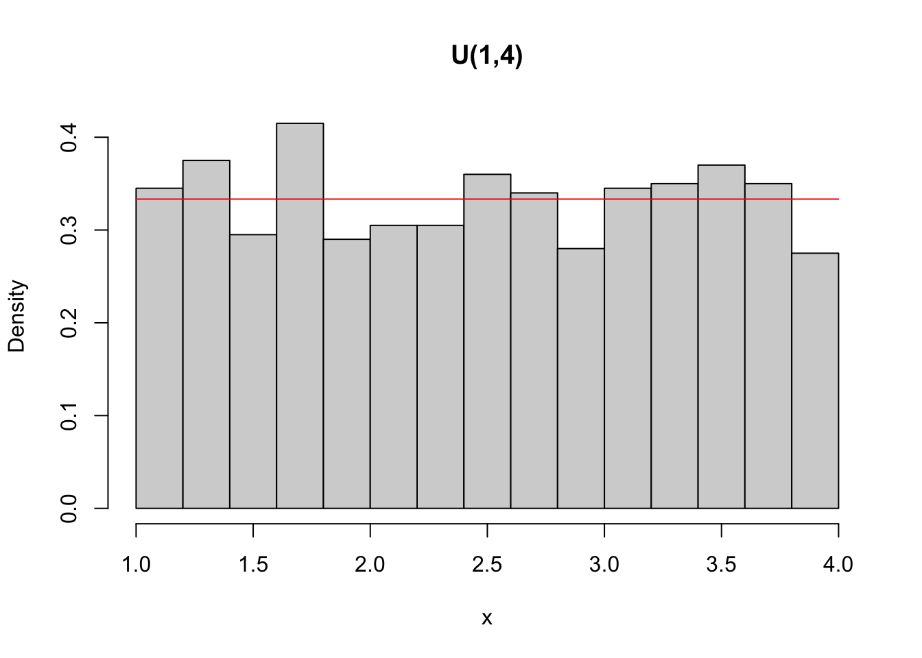
Example 3.37 In Python.
import numpy as np
from scipy.stats import uniform
import matplotlib.pyplot as plt

# P(X < 2) em uma U(1,4)
prob = uniform.cdf(2, loc=1, scale=3)  # scale = 4 - 1 = 3
print(prob)  # Output: 0.3333333333333333

# quantile that limits 2.5% in a U(1,4)
quantil = uniform.ppf(0.025, loc=1, scale=3)
print(quantil)  # Output: 1.075

# simulating 1000 pseudo random values of a U(1,4)
np.random.seed(999)
x = uniform.rvs(size=1000, loc=1, scale=3)
# Statistical summary similar to summary() in R via Pandas
print(pd.Series(x).describe())

# density of a U(1,4), superimposing simulated values
plt.hist(x, density=True, bins='auto', color='lightgray',
         edgecolor='black')
plt.title('U(1,4)')

# Theoretical uniform density curve
x_range = np.linspace(x.min(), x.max(), 100)
plt.plot(x_range, uniform.pdf(x_range,loc=1,scale=3), color='red')

plt.show()3.9.2 Exponential \(\cdot \; \mathcal{E}(\lambda)\)
Consider again the toll described in Section 3.7.4, where on average \(\lambda\) vehicles pass per minute. You can invert the reading, placing the time between each car as the new variable of interest. Thus, 1 car passes through this toll every \(\frac{1}{\lambda}\) minutes. The continuous random variable \(X\): ‘time between vehicles’ has exponential distribution of parameter \(\lambda\), denoted by \[ X \sim \mathcal{E}(\lambda), \] where \(x > 0\) and \(\lambda > 0\) indicates the rate. The exponential density function is given by
\[\begin{equation} f(x|\lambda) = \lambda e^{-\lambda x} \tag{3.78} \end{equation}\] where \(e\) is the Euler’s number. Its cumulative distribution function is given by \[\begin{equation} F(x|\lambda) = Pr(X \le x) = 1 - e^{-\lambda x} \tag{3.79} \end{equation}\] The expected value a nd variance are given by \[\begin{equation} E(X)= \frac{1}{\lambda} = \lambda^{-1} \tag{3.80} \end{equation}\] \[\begin{equation} V(X)=\frac{1}{\lambda^2} = \lambda^{-2} \tag{3.81} \end{equation}\]
Example 3.38 The exponential distribution can be operated with the functions dexp (density), pexp (accumulated probability), qexp (quantile) and rexp (random/random) from the stats library.
## [1] 0.8646647## [1] 0.02531781# simulating 1000 pseudo random values of an exponential of rate 1
set.seed(999); x <- rexp(1000, 1)
summary(x)## Min. 1st Qu. Median Mean 3rd Qu. Max.
## 0.00011 0.29347 0.69805 1.00508 1.41511 5.42528# density of an exponential of rate 1, overlapping simulated values
hist(x, freq = F, ylim = c(0,1), main = 'Exp(1)')
curve(dexp(x,1), add = T, col = 'red')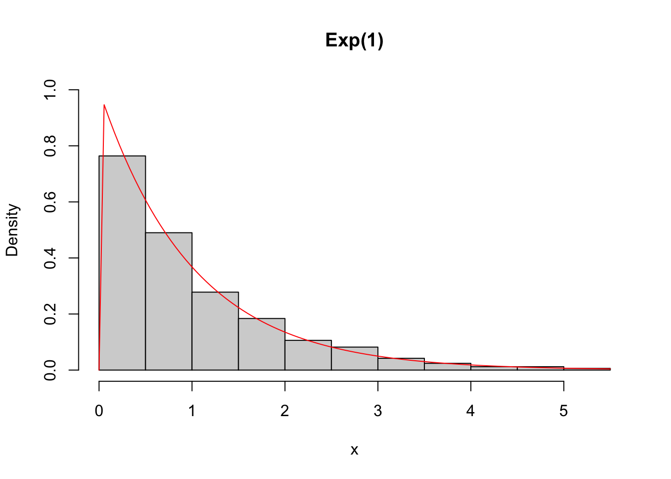
Example 3.39 Consider a tollbooth where an average of \(\lambda = 2\) vehicles pass per minute. Thus, \[ X \sim \mathcal{E}(2),\] \[ f(x) = 2 e^{-2 x}, \] \[ E(X)=\dfrac{1}{2}=0.5, \] \[ V(X)=\dfrac{1}{2^2}=0.25, \] \[ D(X) = \sqrt{0.25} = 0.5. \]
Exercise 3.22 Considering the data from Example 3.39:
a. Define \(F(x)\).
b. Get \(Pr(X<1)\).
c. Obtain \(Pr(X>2)\).
d. Sketch the graph of \(f(x)\).
\(\\\)
3.9.3 Normal \(\cdot \; \mathcal{N}(\mu,\sigma)\)
The normal or Gaussian distribution (named after Johann Carl Friedrich Gauss) is denoted by \(\mathcal{N}(\mu,\sigma)\). Its pdf is given by \[\begin{equation} f(x|\mu,\sigma) = \dfrac{1}{\sqrt{2\pi} \sigma} \exp \bigg\{ -\frac{1}{2} \left( \frac{x-\mu}{\sigma} \right) ^2 \bigg\} \tag{3.82} \end{equation}\]
for \(-\infty < x < \infty\), \(-\infty < \mu < \infty\), \(\sigma > 0\). The parameters \(\mu\) and \(\sigma\) can be calculated respectively by the Equations (2.8) and (2.26). The notation \(\exp\{...\}\) represents the Euler number raised to the expression enclosed by the square brackets.
The standard normal distribution is given by the expression \[\begin{equation} f(z|\mu=0, \sigma=1) = \dfrac{1}{\sqrt{2\pi}} \exp \bigg\{ -\frac{z^2}{2} \bigg\} \tag{3.83} \end{equation}\]
for \(-\infty < z < \infty\).
Example 3.40 The normal distribution can be operated with the functions stats::dnorm() (density), stats::pnorm() (cumulative probability), stats::qnorm() (quantile) and stats::rnorm() (random/random).
## [1] 0.9772499## [1] -1.959964## Min. 1st Qu. Median Mean 3rd Qu. Max.
## -3.073370 -0.705544 -0.009566 -0.032516 0.636537 3.061137# density of a N(0,1), overlapping simulated values
hist(x, freq = F,main = 'N(0,1)')
curve(dnorm(x), add = T, col = 'red')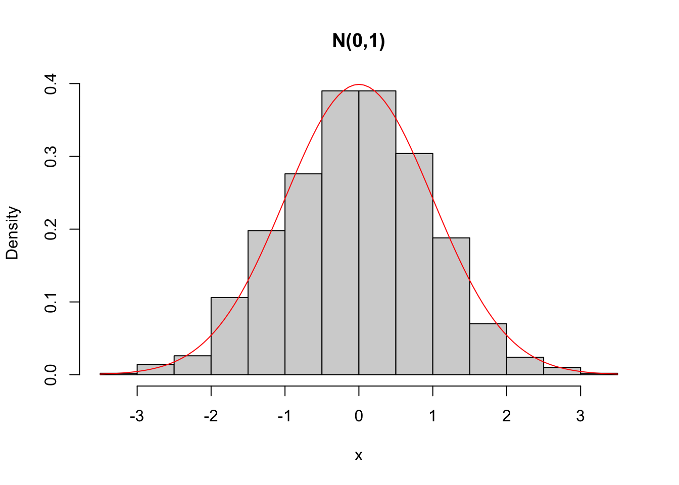
Example 3.41 In Python.
import numpy as np
from scipy.stats import norm
import matplotlib.pyplot as plt

# P(X < 2) em uma N(0,1)
prob = norm.cdf(2)
print(prob)  # Output: 0.9772498680518208

# Quantil que limita 2.5% em uma N(0,1)
quantil = norm.ppf(0.025)
print(quantil)  # Output: -1.959963984540054

# Simulando 1000 valores pseudo aleatórios de uma N(0,1)
np.random.seed(999)
x = np.random.normal(size=1000)
# Resumo estatístico similar ao summary() em R via Pandas
print(pd.Series(x).describe())

# Densidade de uma N(0,1), sobrepondo valores simulados
plt.hist(x, density=True, bins='auto', color='lightgray',
         edgecolor='black')
plt.title('N(0,1)')

# Curva da densidade normal teórica
x_range = np.linspace(x.min(), x.max(), 100)
plt.plot(x_range, norm.pdf(x_range), color='red')

plt.show()
Exercise 3.24 Read the article 68–95–99.7 rule.
3.9.3.1 Central Limit Theorem
The central limit theorem roughly says that the sum of many independent random variables will be approximately normally distributed if each summand has a high probability of being small. (Billingsley 1986, 366)
Theorem 3.2 (Lindeberg–Lévy Central Limit Theorem) Let \(X_{1}, X_{2}, \ldots, X_{n}\) be a sequence of independent random variables with \(E(X_{n}) = \mu\) and \(V(X_{n}) = \sigma^2 < \infty\). Given \(S_n=X_{1}+X_{2}+\ldots+X_{n}\), and if \(n \longrightarrow \infty\), then \[\begin{equation} \frac{S_n - n\mu}{\sigma \sqrt{n}} \xrightarrow{D} \mathcal{N}(0,1). \tag{3.84} \end{equation}\]
Let us then note the difference between the Central Limit Theorem and the Law of Large Numbers [Section ??] in this case. The Law of Large Numbers says that the sample mean \(S_n/n\) converges to \(\mu\), in probability or almost certainly [Section ??], i.e., the difference \(S_n/n - \mu\) tends to zero, and the Central Limit Theorem says that this difference, when multiplied by the square root of \(n\), converges in distribution to a normal one: \(\sqrt{n} \left( \frac{S_n}{n}-\mu \right) \xrightarrow{D} \mathcal{N}(0,\sigma^2).\) (James 2010, 266)
(James 2010,C) points that central is the theorem, not the limit. The origin of the expression is attributed to the Hungarian mathematician George Pólya, when referring to der zentrale Grenzwertsatz, i.e., the ‘central’ refers to the ‘limit theorem’.
Exercise 3.25 Show that Eq. (3.84) can be written in terms of the mean \(M_n=\frac{S_n}{n}\), such that \(\frac{M_n - \mu}{\sigma / \sqrt{n}}\).
Exercise 3.26 Watch the video But what is the Central Limit Theorem? from the channel 3Blue1Brown. I thank Vitor Luiz Cavagnolli Machado for the suggestion.
Exercise 3.27 Consider the random variable \(Z\) with standard normal distribution denoted by \(Z \sim \mathcal{N}(0,1)\). Obtain the following quantities:
a. \(Pr(Z \le -1.96)\).
b. \(Pr(-1 \le Z \le 1)\).
c. \(Pr(Z > 1.64)\).
d. \(q\) tal que \(Pr(Z \le q) = 0.025\).
e. \(q\) tal que \(Pr(-q \le Z \le q) = 0.6826894921\).
f. \(q\) tal que \(Pr(Z > q) = 0.05\).
Solution: Chapter ??
\(\\\)
3.9.3.2 Approximating the binomial by the normal
The proportion is an average in the case where the variable only admits the values 0 and 1, therefore the TCL applies directly to this type of structure. One can also consider a continuity correction, adding 0.5 to the numerator of Equation (3.84).
Example 3.42 (Approximating the binomial by the normal) If we consider \(n=420\) tosses of a coin with \(p=0.5\), we have that the r.v. \(X\): ‘number of heads in 420 tosses’ is such that \(X \sim \mathcal{B}(420,0.5)\). The probability of getting up to 200 heads can be approximated by the TCL. \[ P(X \le 200) \approx P \left( Z < \frac{200-420\times 0.5}{\sqrt{420 \times 0.5 \times 0.5}} \right) = \Phi(-0.9759) \approx 0.164557. \] Using continuity correction, \[ P(X \le 200) \approx P \left( Z < \frac{200+0.5-420\times 0.5}{\sqrt{420 \times 0.5 \times 0.5}} \right) = \Phi(-0.9271) \approx 0.176936. \] With a computer it is possible to calculate the exact probability, notice how close the results are. \[ P(X \le 200) = \left[ \dbinom{420}{0} + \dbinom{420}{1} + \cdots + \dbinom{420}{200} \right] 0.5^{420} \approx 0.1769429. \]
n <- 420
p <- 0.5
S <- 200
mS <- n*p # 210
sS <- sqrt(n*p*(1-p)) # 10.24695
# Binomial approximation by the normal WITHOUT continuity correction
(z <- (S-mS)/sS)
## [1] -0.9759001## [1] 0.164557## [1] -0.9271051## [1] 0.176936## [1] 0.1769429Example 3.43 In Python.
import numpy as np
from scipy.stats import norm, binom

# Parameters of the binomial distribution
n = 420
p = 0.5
S = 200

# Mean and standard deviation of the binomial distribution
mS = n * p # 210
sS = np.sqrt(n * p * (1 - p)) # 10.24695

# Approximation of the binomial by the normal WITHOUT continuity correction
z = (S - mS) / sS
prob_sem_correcao = norm.cdf(z)
print(prob_sem_correcao) # Output: 0.1668580917315335

# Approximation of the binomial by the normal WITH continuity correction
zc = (S + 0.5 - mS) / sS
prob_com_correcao = norm.cdf(zc)
print(prob_com_correcao) # Output: 0.1715144436436775

# Exact probability
prob_exata = binom.cdf(S, n, p)
print(prob_exata) # Output: 0.1713874634776793
3.9.3.3 Learn more
(Patel and Read 1982) provides a collection of results and properties related to the normal distribution. (Tong 1990) provides a comprehensive treatment of results related to the multivariate normal distribution. The main topics are dependence, probability inequalities, and their roles in theory and applications.
3.9.4 Chi-squared \(\cdot \; \mathcal{\chi}^2_\nu\)
If \(X \sim \chi^2_\nu\), then its pdf is given by
\[\begin{equation} f(x|\nu) = \frac{1}{\Gamma \left( \frac{\nu}{2} \right) 2^{\nu/2}} x^{\frac{\nu}{2}-1} e^{-\frac{x}{2}} \tag{3.85} \end{equation}\]
where \(x > 0\), \(\nu > 0\) indicates the degrees of freedom and \(\Gamma\) is the gamma function according to Eq. (3.88). Equivalently, one can write down \(X \sim \chi^2(\nu)\).
Example 3.44 The \(\chi^2\) distribution can be operated with the functions dchisq (density), pchisq (accumulated probability), qchisq (quantile) and rchisq (random/random) from the stats library.
## [1] 0.8427008## [1] 0.0009820691# simulating 1000 pseudo random values from a \chi^2 with 1 df
set.seed(135); x <- rchisq(1000, gl)
summary(x)## Min. 1st Qu. Median Mean 3rd Qu. Max.
## 0.00000 0.08634 0.42728 0.98606 1.30768 8.91451# density of a \chi^2 with 1 degree of freedom, overlapping simulated values
hist(x, 50, freq = F, main = bquote(chi^2~ (.(gl))))
curve(dchisq(x,1), 0, 10, add = T, col = 'red')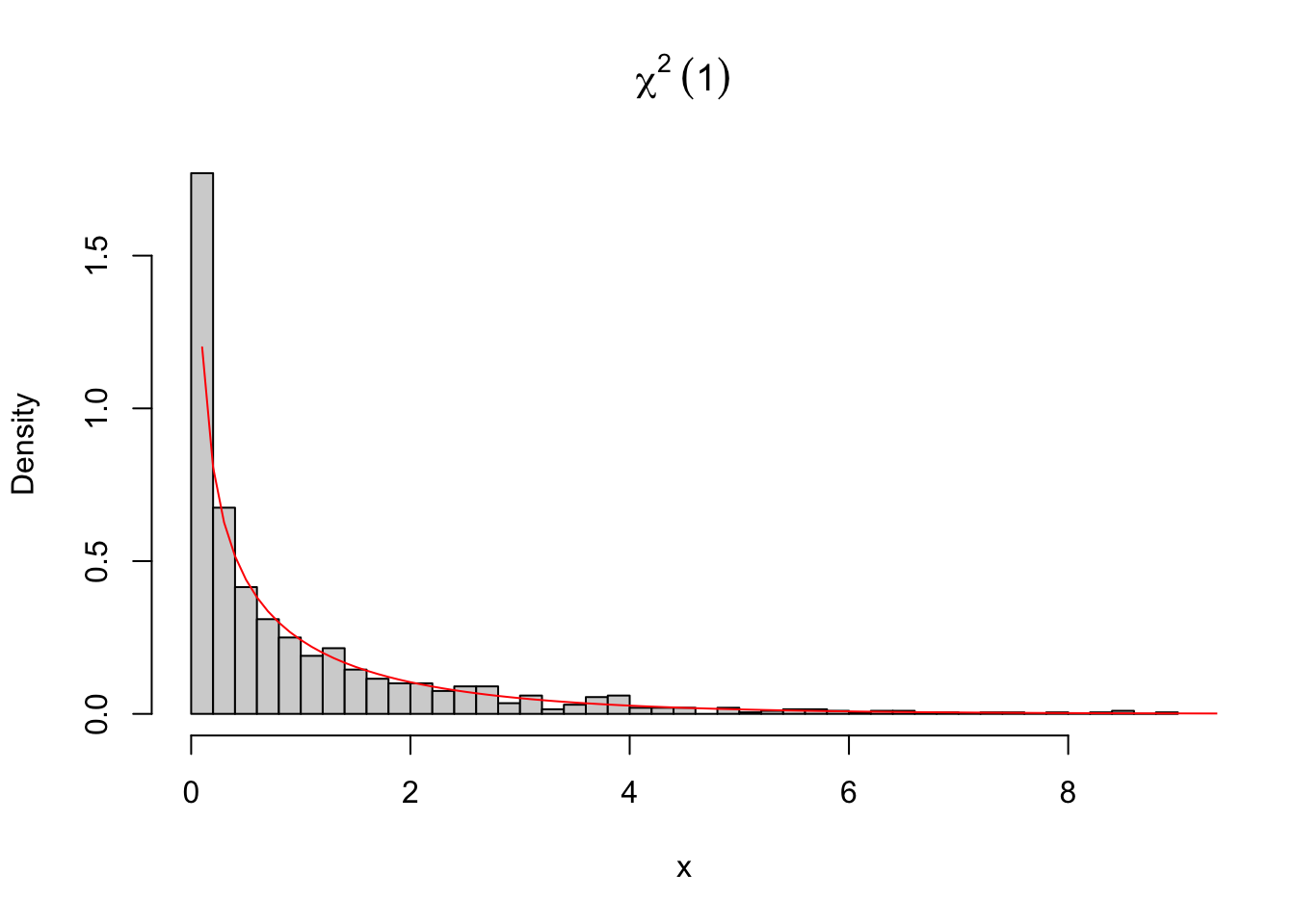
Characterization
\(Q \sim \chi^2_\nu\) if
\[\begin{equation} Q = \sum_{i=1}^\nu Z_i^2 \tag{3.86} \end{equation}\]
where \(Z_i^2 \sim \mathcal{N}(0,1)\), \(i \in \{1,\ldots,\nu\}\).
Example 3.45 It is possible to simulate a chi-square with 1 degree of freedom.
# via standard normal squared
set.seed(1234); q1 <- rnorm(1000)^2
# via rchisq
set.seed(5678); q2 <- rchisq(1000, 1)
par(mfrow=c(1,2))
hist(q1, 30)
hist(q2, 30)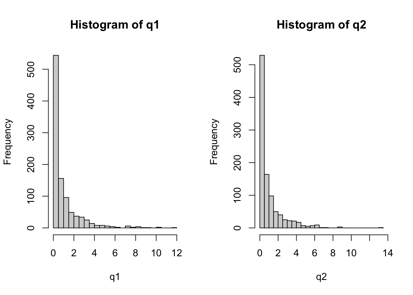
##
##  Asymptotic two-sample Kolmogorov-Smirnov test
##
## data:  q1 and q2
## D = 0.026, p-value = 0.8879
## alternative hypothesis: two-sided
Exercise 3.28 Simulate a chi-square with 3 degrees of freedom via Eq. (3.86). Compare with the simulation obtained via rchisq.
3.9.5 Student’s \(t\) \(\cdot \; \mathcal{t_\nu}\)
The continuous random variable \(X\) has a Student’s \(t\) distribution with \(\nu\) degrees of freedom, denoted by \(X \sim t(\nu)\), if its density function is given by
\[\begin{equation} f(x|\nu) = \frac{\Gamma \left( \frac{\nu+1}{2} \right)}{\Gamma \left( \frac{\nu}{2} \right) \sqrt{\nu \pi}} \left( 1+\frac{x^2}{\nu} \right)^{-\frac{\nu + 1}{2}} \tag{3.87} \end{equation}\]
where \(-\infty < x < \infty\), \(\nu > 0\) indicates the degrees of freedom and \(\Gamma\) indicates the gamma function such that
\[\begin{equation} \Gamma(x) = \int_{0}^{\infty} t^{x-1} e^{-t} dt \tag{3.88} \end{equation}\]
Equivalently, one can write down \(X \sim t(\nu)\).
Example 3.46 The \(t\) distribution can be operated with the functions stats::dt() (density), stats::pt() (accumulated probability), stats::qt() (quantile) and stats::rt() (random/random).
## [1] 0.8524164## [1] -12.7062# simulating 1000 pseudo random values from a t with 1 df
set.seed(246); x <- rt(1000, 1)
summary(x)## Min. 1st Qu. Median Mean 3rd Qu. Max.
## -305.1952 -1.1336 -0.0891 0.3420 1.0430 1294.5135# density of a t with 1 degree of freedom, overlapping simulated values
hist(x, 3000, freq = F, xlim = c(-15,15), main = expression(italic('t')(1)))
curve(dt(x,1), add = T, col = 'red')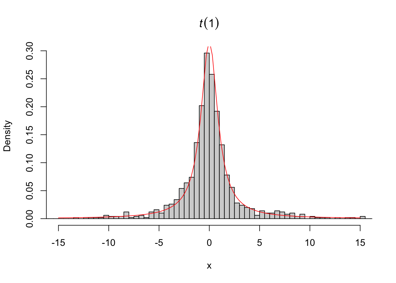
Example 3.47 In Python.
import numpy as np
from scipy.stats import t
import matplotlib.pyplot as plt

# Pr(X < 2) em uma t com 1 gl
prob = t.cdf(2, df=1)
print(prob)  # Output: 0.8524163823517757

# Quantil que limita 2.5% em uma t com 1 gl
quantil = t.ppf(0.025, df=1)
print(quantil)  # Output: -12.706204736174703

# Simulando 1000 valores pseudo aleatórios de uma t com 1 gl
np.random.seed(246)
x = t.rvs(size=1000, df=1)
# Resumo estatístico similar ao summary() em R via Pandas
print(pd.Series(x).describe())

# Densidade de uma t com 1 gl, sobrepondo valores simulados
plt.hist(x, density=True, bins=3000, color='lightgray',
         edgecolor='black')
plt.xlim(-15, 15)  # Definindo o limite do eixo x
# Usando expressão matemática LaTeX para o título
plt.title(r'$t(1)$', fontsize=16)

# Curva da densidade t teórica
x_range = np.linspace(-15, 15, 1000)
plt.plot(x_range, t.pdf(x_range, df=1), color='red')

plt.show()
3.9.5.1 Characterization
According to (Johnson, Kotz, and Balakrishnan 1995, 2:362),
\[\begin{equation} t(\nu) = Z \left[ \frac{\chi^2(\nu)}{\nu} \right]^{-1/2} \tag{3.89} \end{equation}\]
where \(Z \sim \mathcal{N}(0,1)\).
3.9.6 Fisher-Snedecor \(\cdot \; \mathcal{F}_\nu\)
If \(X \sim \mathcal{F}_{\nu_1,\nu_2}\), then its pdf is given by
\[\begin{equation} f(x|\nu_1,\nu_2) = \frac{\sqrt{\frac{(\nu_1 x)^{\nu_1} \nu_2^{\nu_2}}{(\nu_1 x+\nu_2)^{\nu_1 + \nu_2}}}}{x B\left( \frac{\nu_1}{2}, \frac{\nu_2}{2} \right)} \tag{3.90} \end{equation}\]
where \(x > 0\), \(\nu_1 > 0\) indicates the numerator degrees of freedom, \(\nu_2 > 0\) indicates the denominator degrees of freedom and \(B\) indicates the beta function, such that
\[\begin{equation} B(x_1,x_2) = \int_{0}^{1} t^{x_1 - 1} (1-t)^{x_2 - 1} dt = \frac{\Gamma(x_1) \Gamma(x_2)}{\Gamma(x_1+x_2)} \tag{3.91} \end{equation}\]
Example 3.48 The distribution \(\mathcal{F}\) can be operated with the functions df (density), pf (cumulative probability), qf (quantile) and rf (random/random) from the library stats.
# Pr(X < 2) in an F with 1 df in the numerator and 3 df in the denominator
gl1 <- 1
gl2 <- 3
pf(2, gl1, gl2)
## [1] 0.7477845## [1] 0.001157189#simulating 1000 pseudo-random values of an F(1,3)
set.seed(1010); x <- rf(1000, gl1, gl2)
summary(x)## Min. 1st Qu. Median Mean 3rd Qu. Max.
## 0.0000 0.1073 0.5564 2.3601 1.9758 120.0880# density of an F(1,3), overlapping simulated values
hist(x, 500, freq = F, xlim = c(0,10), main = bquote(F(.(gl1),.(gl2))))
curve(df(x, gl1, gl2), 0, 10, add = TRUE, col = 'red')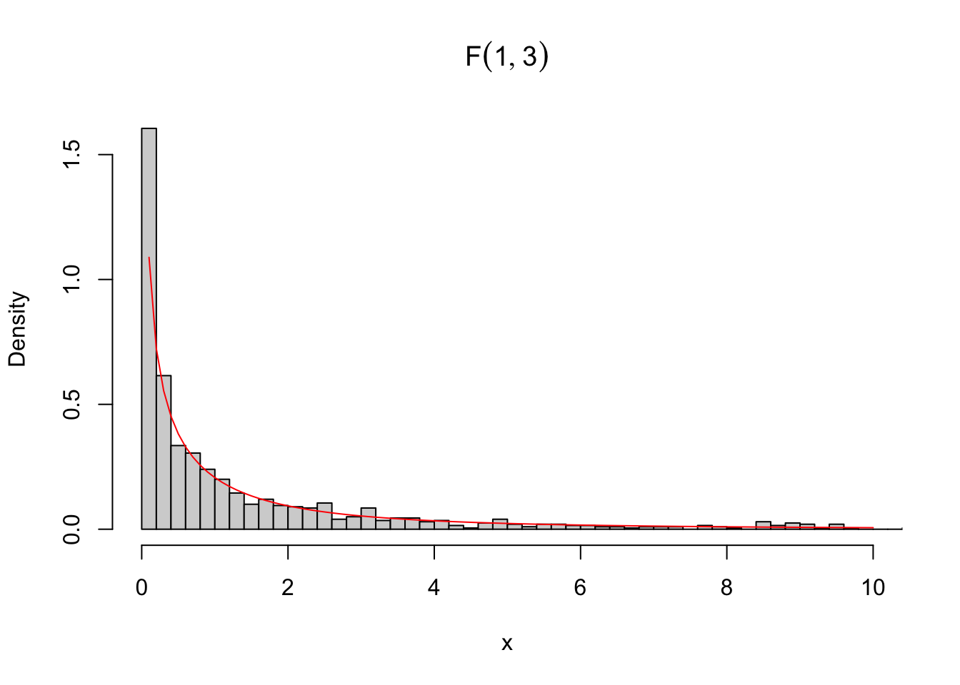
Characterization
\(X \sim \mathcal{F}_{\nu_1,\nu_2}\) if
\[\begin{equation} X = \frac{Q_1/\nu_1}{Q_2/\nu_2} \tag{3.92} \end{equation}\]
where \(Q_1 \sim \chi^2_{\nu_1}\) and \(Q_2 \sim \chi^2_{\nu_2}\).
Example 3.49 It is possible to simulate a \(\mathcal{F}\) with \(\nu_1=1\) degree of freedom in the numerator and \(\nu_2=3\) degrees of freedom in the denominator.
set.seed(1234); q1 <- rchisq(1000, 1)
set.seed(5678); q2 <- rchisq(1000, 3)
x1 <- (q1/1)/(q2/3)
x2 <- rf(1000, 1, 3)
par(mfrow=c(1,2))
hist(x1, 50, xlim = c(0,20))
hist(x2, 100, xlim = c(0,20))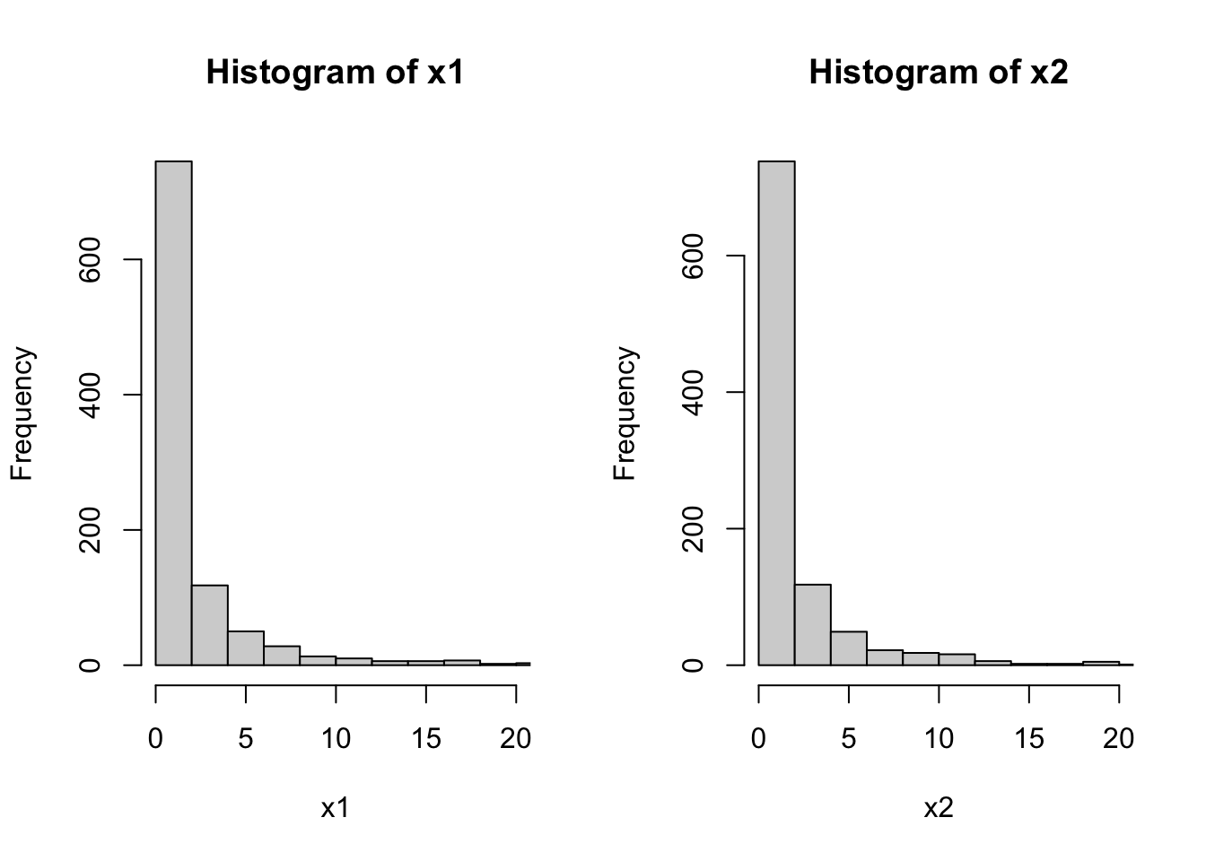
##
##  Asymptotic two-sample Kolmogorov-Smirnov test
##
## data:  x1 and x2
## D = 0.023, p-value = 0.9541
## alternative hypothesis: two-sided
3.9.7 Beta \(\cdot \; \mathcal{Beta}(\alpha,\beta)\)
The beta density function is given by \[\begin{equation} f(x|\alpha,\beta) = \dfrac{\Gamma(\alpha+\beta)}{\Gamma(\alpha)\Gamma(\beta)} x^{\alpha-1} (1-x)^{\beta-1} \tag{3.93} \end{equation}\] where \(0 \le x \le 1\), \(\alpha,\beta > 0\) and \(\Gamma\) is the gamma function according to Eq. (3.88). Expected value and variance are given by \[\begin{equation} E(X) = \frac{\alpha}{\alpha+\beta} \tag{3.94} \end{equation}\] \[\begin{equation} V(X) = \frac{\alpha\beta}{(\alpha+\beta)^2 (\alpha+\beta+1)} \tag{3.95} \end{equation}\]
The median and mode are given by \[\begin{equation} Md(X) \approx \frac{\alpha-1/3}{\alpha+\beta-2/3} \tag{3.96} \end{equation}\] \[\begin{equation} Mo(X) = \frac{\alpha-1}{\alpha+\beta-2}, \; \alpha,\beta>1 \tag{3.97} \end{equation}\] \[\begin{equation} Mo(X) \; \text{algum valor entre 0 e 1}, \; \alpha=\beta=1 \tag{3.98} \end{equation}\] \[\begin{equation} Mo(X) = \{0,1\}, \; \alpha,\beta<1 \tag{3.99} \end{equation}\] \[\begin{equation} Mo(X) = 0, \; \alpha \le 1,\beta>1 \tag{3.100} \end{equation}\] \[\begin{equation} Mo(X) = 1, \; \alpha>1,\beta \le 1 \tag{3.101} \end{equation}\]
Example 3.50 The Beta distribution can be operated with the functions dbeta (density), pbeta (cumulative probability), qbeta (quantile) and rbeta (random/random) from the stats library.
## [1] 0.875## [1] 0.008403759# simulating 1000 pseudo random values of a Beta(1,3)
set.seed(1010); x <- rbeta(1000, 1, 3)
summary(x)## Min. 1st Qu. Median Mean 3rd Qu. Max.
## 0.0000842 0.0905449 0.2126896 0.2502407 0.3621014 0.9394182# density of a Beta(1,3), overlaying simulated values
hist(x, 30, freq = F, ylim = c(0, 3), main = 'Beta(1,3)')
curve(dbeta(x,1,3), add = T, col = 'red')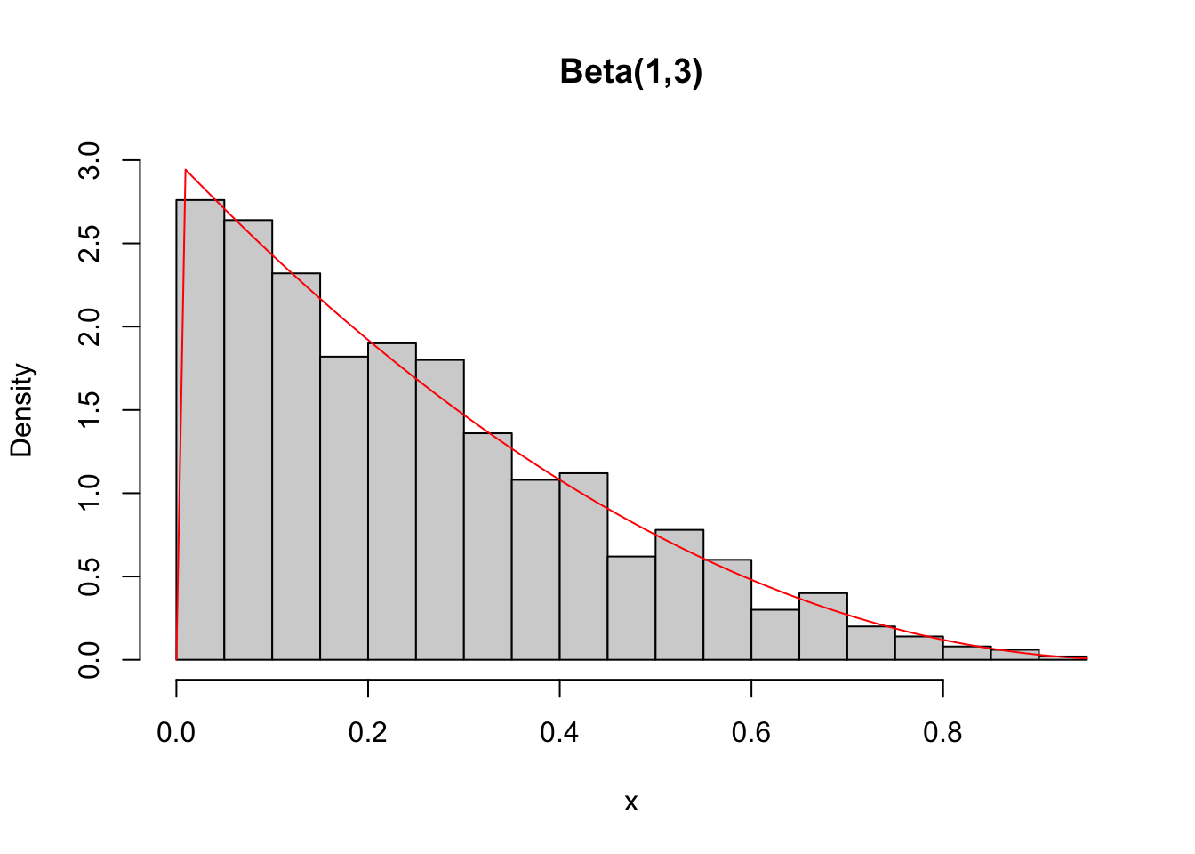
3.9.8 Gamma \(\cdot \; \mathcal{Gama}(k,g)\)
The gamma density function can be given by \[\begin{equation} f(x|k,g) = \frac{1}{\Gamma(k) g^k} x^{k-1} e^{-\frac{x}{g}} \tag{3.102} \end{equation}\] where \(x>0\), \(k>0\) (shape), \(g>0\) (scale) and \(\Gamma\) is the gamma function according to Eq. (3.88). Expected value and variance are given by \[\begin{equation} E(X) = kg \tag{3.103} \end{equation}\] \[\begin{equation} V(X) = kg^2 \tag{3.104} \end{equation}\]
The median does not have a closed form, and the mode is given by \[\begin{equation} Mo(X) = (k-1)g, \;\; k \ge 1 \tag{3.105} \end{equation}\] \[\begin{equation} Mo(X) = 0, \;\; k < 1 \tag{3.105} \end{equation}\]
Example 3.51 The Gamma distribution can be operated with the functions dgamma (density), pgamma (accumulated probability), qgamma (quantile) and rgamma (random/random) from the stats library.
## [1] 0.9975212## [1] 0.008439269# simulating 1000 pseudo-random values of a Gamma(1,3)
set.seed(1010); x <- rgamma(1000, 1, 3)
summary(x)## Min. 1st Qu. Median Mean 3rd Qu. Max.
## 0.0003625 0.0914895 0.2279837 0.3381387 0.4639010 2.6271045# density of a Gamma(1,3), overlapping simulated values
hist(x, 30, freq = F, ylim = c(0, 3), main = 'Gama(1,3)')
curve(dgamma(x,1,3), add = T, col = 'red')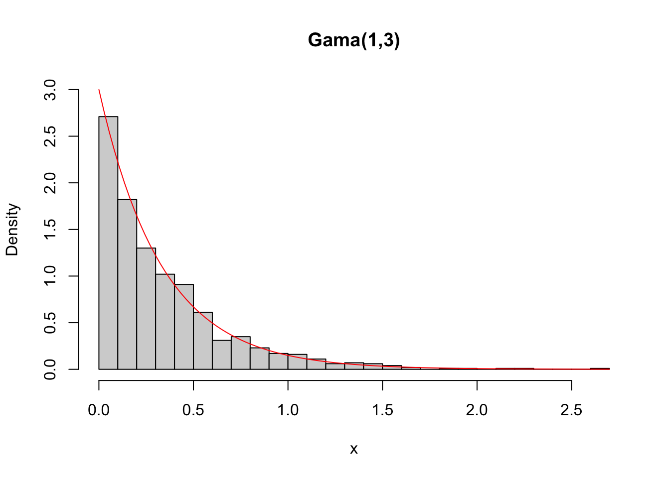
3.9.9 Triangular \(\cdot \; \mathcal{Tri}(a,m,b)\)
(Samuel Kotz and Van Dorp 2004) define the triangular density function in the interval \([a,b]\) with mode \(m\) by \[\begin{equation} f(x|a,b,m) = \left\{ \begin{array}{l} \frac{2}{b-a} \frac{x-a}{m-a}, \;\; a \le x \le m \\ \frac{2}{b-a} \frac{b-x}{b-m}, \;\; m < x \le b \\ \end{array} \right. \tag{3.107} \end{equation}\]
where \(a \le x \le b\) e \(a \le m \le b\), \(-\infty < a,b < \infty\) with \(b>a\).
Its cumulative distribution function is given by \[\begin{equation} F(x|a,b,m) = Pr(X \le x) = \left\{ \begin{array}{l} \frac{m-a}{b-a} \left( \frac{x-a}{m-a} \right)^2, \;\; a \le x \le m \\ 1 - \frac{b-m}{b-a} \left( \frac{b-x}{b-m} \right)^2, \;\; m < x \le b \\ \end{array} \right. \tag{3.108} \end{equation}\]
Its inverse cumulative distribution function is given by \[\begin{equation} F^{-1}(u|a,b,m) = \left\{ \begin{array}{l} a + \sqrt{u(m-a)(b-a)}, \;\; 0 \le u \le \frac{m-a}{b-a} \\ b - \sqrt{(1-u)(b-m)(b-a)}, \;\; \frac{m-a}{b-a} < u \le 1 \\ \end{array} \right. \tag{3.109} \end{equation}\]
(Millard 2013) presents the EnvStats package, which has varied functions for Environmental Statistics that consider the triangular distribution.
library(EnvStats)
set.seed(2); hist(rtri(10000), 40, freq = FALSE, main = 'Tri(0,1/2,1)')
curve(dtri(x), col = 'red', add = TRUE)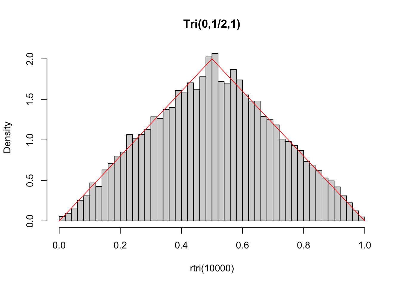
Exercise 3.30 See the documentation for ?EnvStats::dtri.
3.9.10 Gompertz \(\cdot \; \mathcal{Gompertz}(\alpha,\beta)\)
(Gompertz 1825) defines the Gompertz density function of shape parameter \(\alpha>0\) and scale \(\beta>0\) for \(x>0\) by \[\begin{equation} f(x|\alpha,\beta) = \alpha \beta \exp \left\{ \beta x + \alpha - \alpha e^{\beta x} \right\} \tag{3.110} \end{equation}\]
Its cumulative distribution function is given by \[\begin{equation} F(x|\alpha,\beta) = 1 - \exp \left\{ - \alpha(e^{\beta x}-1) \right\} \tag{3.111} \end{equation}\]
(Yee 2010) presents functions for the Gompertz distribution.
library(VGAM)
curve(dgompertz(x, scale = 1, shape = .1), xlim = c(0,5), ylim = c(0,1.2),
      col = 'red')
curve(dgompertz(x, scale = 1, shape = 2), xlim = c(0,5), ylim = c(0,1.2),
      col = 'black', add = TRUE)
curve(dgompertz(x, scale = 1, shape = 3), xlim = c(0,5), ylim = c(0,1.2),
      col = 'blue', add = TRUE)
curve(dgompertz(x, scale = 2, shape = 1), xlim = c(0,5), ylim = c(0,1.2),
      col = 'green', add = TRUE)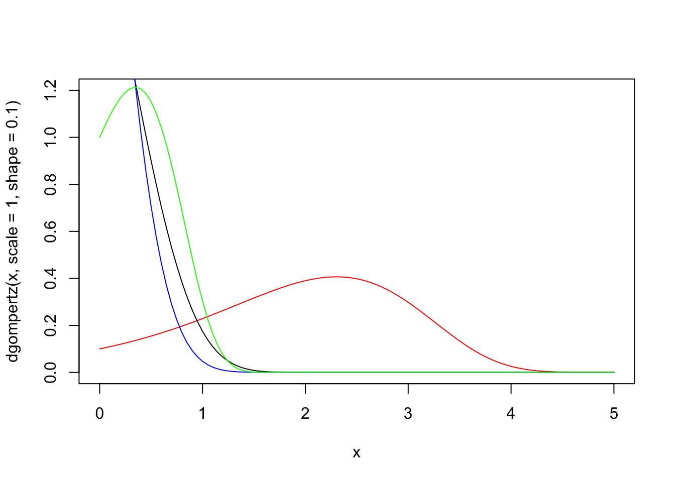
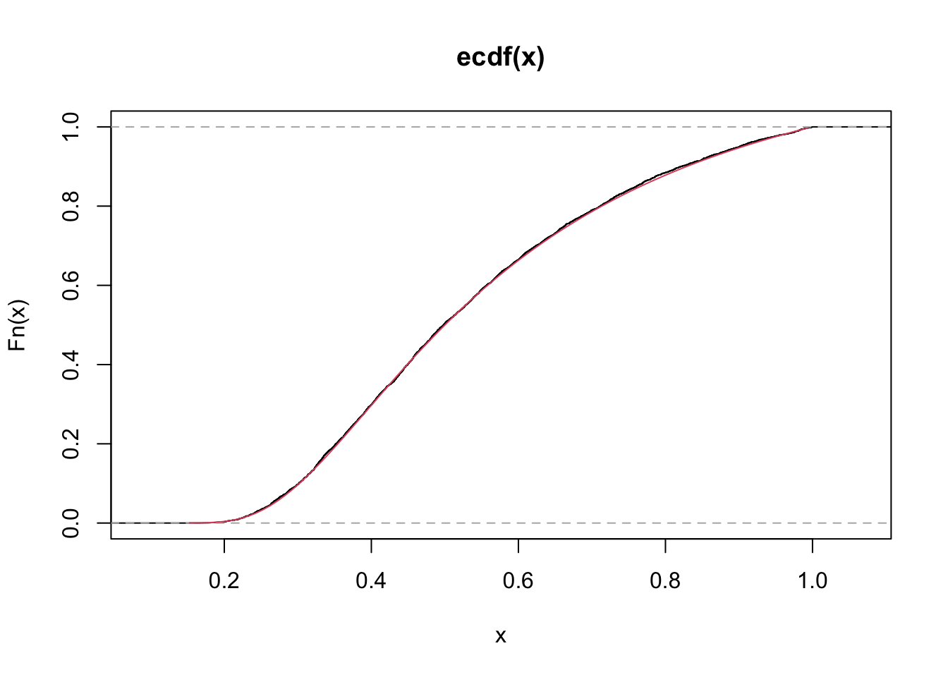
3.9.11 Unit-Gompertz \(\cdot \; \mathcal{GU}(\alpha,\beta)\)
(Mazucheli, Menezes, and Dey 2019) define the Unit-Gompertz distribution from the type transformation \[X=e^{-Y}\]
where \(Y\) has a Gompertz distribution. Its density function with parameters \(\alpha>0\) and \(\beta>0\) with \(0<x<1\) is given by
\[\begin{equation} f(x|\alpha,\beta) = \alpha \beta x^{-(\beta+1)} \exp \left\{ -\alpha(x^{-\beta}-1) \right\} \tag{3.112} \end{equation}\]
Its cumulative distribution function is given by \[\begin{equation} F(x|\alpha,\beta) = \exp \left\{ -\alpha(x^{-\beta}-1) \right\} \tag{3.113} \end{equation}\]
(Menezes and Mazucheli 2021) present the unitquantreg package, that provides a collection of parametric quantile regression models for bounded data. The autors also present functions for the unit-Gompertz distribution reparametrized in terms of the \(\tau\)-th quantile, \(\tau \in (0,1)\).
library(unitquantreg)
set.seed(123)
x <- rugompertz(n = 5000, mu = 0.5, theta = 2, tau = 0.5)
R <- range(x)
S <- seq(from = R[1], to = R[2], by =  0.01)
hist(x, prob = TRUE, main = 'Gompertz unit')
lines(S, dugompertz(x = S, mu = 0.5, theta = 2, tau = 0.5), col = 2)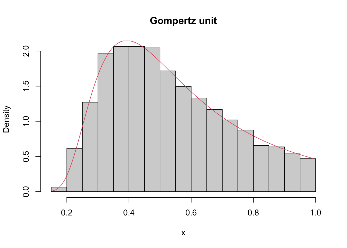
plot(quantile(x, probs = S), type = "l")
lines(qugompertz(p = S, mu = 0.5, theta = 2, tau = 0.5), col = 2)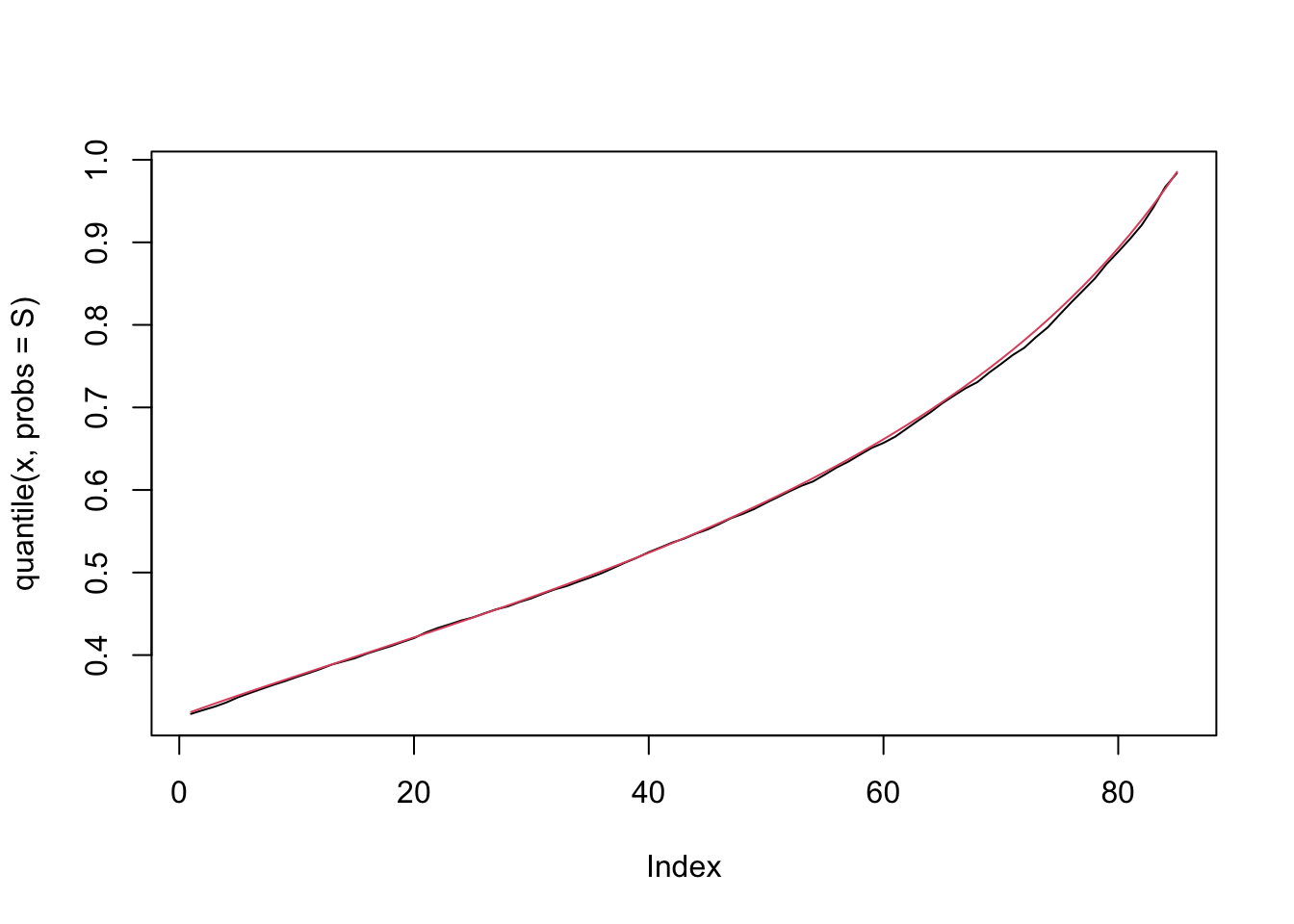
3.9.12 Continuous Poisson
(Ilienko 2013) presents and discusses continuous counterparts of the Poisson and binomial distributions.