3.3 Definitions
3.3.1 Random experiment
Definition 3.2 A (random) experiment is a procedure that can be performed infinitely many times under the same conditions, associated with a set of all possible outcomes (sample space).
3.3.2 Sample space
Definition 3.3 The sample space is the set of all possible outcomes of a random experiment, symbolized by \(\Omega\).
Example 3.12 (Finite sample space 1) In the case of the random experiment ‘throwing a die’, the sample space is defined by \[ \Omega = \left\lbrace 1, 2, 3, 4, 5, 6 \right\rbrace. \]
Exercise 3.3 Access the link http://a.teall.info/dice/.
a. Describe the sample space for each of the data individually.
b. Describe the sample space considering rolling 2 4-sided dice (2d4).
c. Describe the sample space considering rolling 1 4-sided die (d4) and 1 6-sided die (d6).
Solution: Chapter 8
\(\\\)
Example 3.13 (Finite sample space 2) The random experiment ‘throwing a die twice’ is equivalent to ‘throwing two dice (with the same configuration)’. The sample space is defined by \[ \Omega = \left\lbrace \begin{array}{cccccc} (1,1) & (1,2) & (1,3) & (1,4) & (1,5) & (1,6) \\ (2,1) & (2,2) & (2,3) & (2,4) & (2,5) & (2,6) \\ (3,1) & (3,2) & (3,3) & (3,4) & (3,5) & (3,6) \\ (4,1) & (4,2) & (4,3) & (4,4) & (4,5) & (4,6) \\ (5,1) & (5,2) & (5,3) & (5,4) & (5,5) & (5,6) \\ (6,1) & (6,2) & (6,3) & (6,4) & (6,5) & (6,6) \\ \end{array} \right\rbrace \]
Example 3.14 (Infinite sample space) In Example 2.8, the sample space is defined by the uncountable set \(\Omega = \lbrace b \in \mathbb{R} : 0 \le b\le 1 \ rbrace\).
3.3.3 Event
Definition 3.4 An event is a subset of the sample space.
Example 3.15 (Finite event) From Example 3.12 one may only be interested in the even results of the toss. So the ‘even face’ event can be described as \(E = \left\lbrace 2,4,6 \right\rbrace\). Note that \(E \subset \Omega\). \(\\\)
Definition 3.5 Events \(A\) and \(B\) are mutually exclusive or disjoint if \(A\) and \(B\) cannot occur simultaneously, i.e., \(A \cap B = \emptyset\).
Definition 3.6 Events \(A_1,A_2,\ldots,A_k\) are collectively exhaustive if at least one of the events must occur, i.e., \(\cup_{i =1}^{k} A_i=\Omega\).
Example 3.16 From the Example 3.12 we can consider \(E = \left\lbrace 2,4,6 \right\rbrace\) (even face) and \(F = \left\lbrace 1,3,5 \right \rbrace\) (odd face). These events are mutually exclusive since \(E \cap F = \emptyset\) and collectively exhaustive since \(E \cup F = \Omega\).
3.3.4 Probability
One can assign the probability of event \(A\) as
\[\begin{equation} Pr(A)=\frac{m}{n} \tag{3.20} \end{equation}\]
where
- \(m\) is the number of favorable cases for the event \(A\)
- \(n\) is the total number of cases
The frequentist probability is the limit of Equation (3.20) when \(n \rightarrow \infty\). If the probability of the event \(A\) represents a reasonable expectation (Cox 1946), a state of knowledge (Jaynes 1985) or the quantification of a personal belief (De Finetti 1970), we call subjective probability.
Example 3.17 (Frequent probability) Suppose a die is rolled 150 times, and observe the distribution of rolls shown in the following table.
| Side | \(1\) | \(2\) | \(3\) | \(4\) | \(5\) | \(6\) | Total |
|---|---|---|---|---|---|---|---|
| Frequency | \(18\) | \(24\) | \(34\) | \(26\) | \(27\) | \(21\) | \(150\) |
Thus, the sample space is \(\Omega = \left\lbrace 1, 2, 3, 4, 5, 6 \right\rbrace\) and one can calculate some probabilities such as \[ Pr(\text{Side 2}) = Pr(\left\lbrace 2 \right\rbrace) = \frac{24}{150} = 0.16 = 16\%\] \[ Pr(\text{Even number}) = Pr(\left\lbrace 2 \right\rbrace \cup \left\lbrace 4 \right\rbrace \cup \left\lbrace 6 \right\rbrace) = \frac{24+26+21}{150} = \frac{71}{150} \approx 0.4733 = 47.33\% \] \[ Pr(\text{Odd number}) = 1-Pr(\text{Face par})=1-\frac{71}{150}=\frac{79}{150} \approx 0.5267=52.67\% \] \[ Pr(\text{Side 2 and side 4 and side 6}) = Pr(\left\lbrace 2 \right\rbrace \cap \left\lbrace 4 \right\rbrace \cap \left\lbrace 6 \right\rbrace) = Pr(\emptyset) =0 \]
## [1] 0.16## [1] 0.4733333## [1] 0.5266667## [1] 71/150## [1] 79/150Exercise 3.4 See the video Deadliest Animal Comparison: Probability and Rate of Death from the channel Reigarw Comparisons, which presents a comparison of deadliest animals. See also sources. Considering independent events, calculate the probability that a person dies:
a. Attacked by a dog.
b. Murdered by someone else.
c. Bitten by a mosquito.
d. Attacked by a dog, murdered by someone else, or bitten by a mosquito.
e. If there are approximately 8 billion people on planet Earth, how many people are expected to die from the causes described in parts a, b, c, and d?
Solution: Chapter 8 \(\\\)
3.3.5 Fundamental properties (Kolmogorov axioms)
For more details, (Kolmogorov 1956), (Feller 1968) and (James 2010) are recommended.
- P1
\[\begin{equation} 0 \le Pr(A) \le 1 \tag{3.21} \end{equation}\] - P2
\[\begin{equation} Pr(\Omega)=1 \tag{3.22} \end{equation}\] - P3 If \(A_1\), \(A_2\), …, \(A_k\) are disjoint sets, then \[\begin{equation} Pr(A_1 \cup A_2 \cup \ldots \cup A_k) = Pr(A_1) + Pr(A_2) + \ldots + Pr(A_k) \tag{3.23} \end{equation}\]
Exercise 3.5 In the classic O Homem que Calculava (Tahan 1938), the protagonist Beremiz Samir solves a problem in which 35 camels should be divided among three brothers in the following proportion: the eldest (\(A\)) would have half of the camels, the brother the middle (\(B\)) with 1/3 and the youngest (\(C\)) with 1/9.
a. Beremiz Samir solved the problem by putting one more camel in the division, resulting in \(\frac{36}{2} = 18\) camels for \(A\), \(\frac{36}{3} = 12\) for \(B\) and \(\frac{36}{9} = 4\) to \(C\), leaving two camels. Explain how this occurs. Hint: 35 %% 3.
b. Check that this problem violates Kolmogorov’s second axiom.
Solution: Chapter 8 \(\\\)
3.3.6 Secondary properties
From the fundamental properties result other, presented without demonstration:
P4 (Complement)
\[\begin{equation} Pr(A)=1-Pr(A^C) \tag{3.24} \end{equation}\]P5
\[\begin{equation} Pr(\emptyset)=0 \tag{3.25} \end{equation}\]P6
If \(A\) and \(B\) are two different sets, then \[\begin{equation} Pr(A \cup B) = Pr(A) + Pr(B) - Pr(A \cap B) \tag{3.26} \end{equation}\]P7 (De Morgan’s Law 1, Eq. (3.13))
\[\begin{equation} Pr(\left[ A \cup B \right]^C) = Pr(A^C \cap B^C) \tag{3.27} \end{equation}\]P8 (De Morgan’s Law 2, Eq. (3.14))
\[\begin{equation} Pr(\left[ A \cap B \right]^C) = Pr(A^C \cup B^C) \tag{3.28} \end{equation}\]
Example 3.18 In a group of \(n\) people, \(2 \le n \le 365\), the probability of the event \(A\): ‘at least two people have birthdays on the same day and month’ can be calculated by the complement property. Considering a year of 365 equiprobable days as indicated by (Feller 1968, 33) and without the presence of twins, triplets, etc., the probability of the event \(A^C\): ‘no person has a birthday on the same day and month as another’, is \[\begin{equation} Pr(A^C) = \frac{365}{365} \times \frac{364}{365} \times \frac{363}{365} \times \cdots \times \frac{365-n+1}{365} \tag{3.29} \end{equation}\] Therefore, \[\begin{equation} Pr(A) = 1 - \left( \frac{365}{365} \times \frac{364}{365} \times \frac{363}{365} \times \cdots \times \frac{365-n+1}{365} \right) \tag{3.30} \end{equation}\]
## [1] 0.5072972prob <- sapply(1:100, birthday)
plot(1:100, prob, main = 'Pr(A)', xlab = '', las = 1)
points(c(23, 41, 57), c(birthday(23), birthday(41), birthday(57)), pch = 16, col = 'red')
legend(19, 0.55, '(23, 0.5073)', bty = 'n')
legend(35, 0.91, '(41, 0.9032)', bty = 'n')
legend(51, 0.99, '(57, 0.9901)', bty = 'n')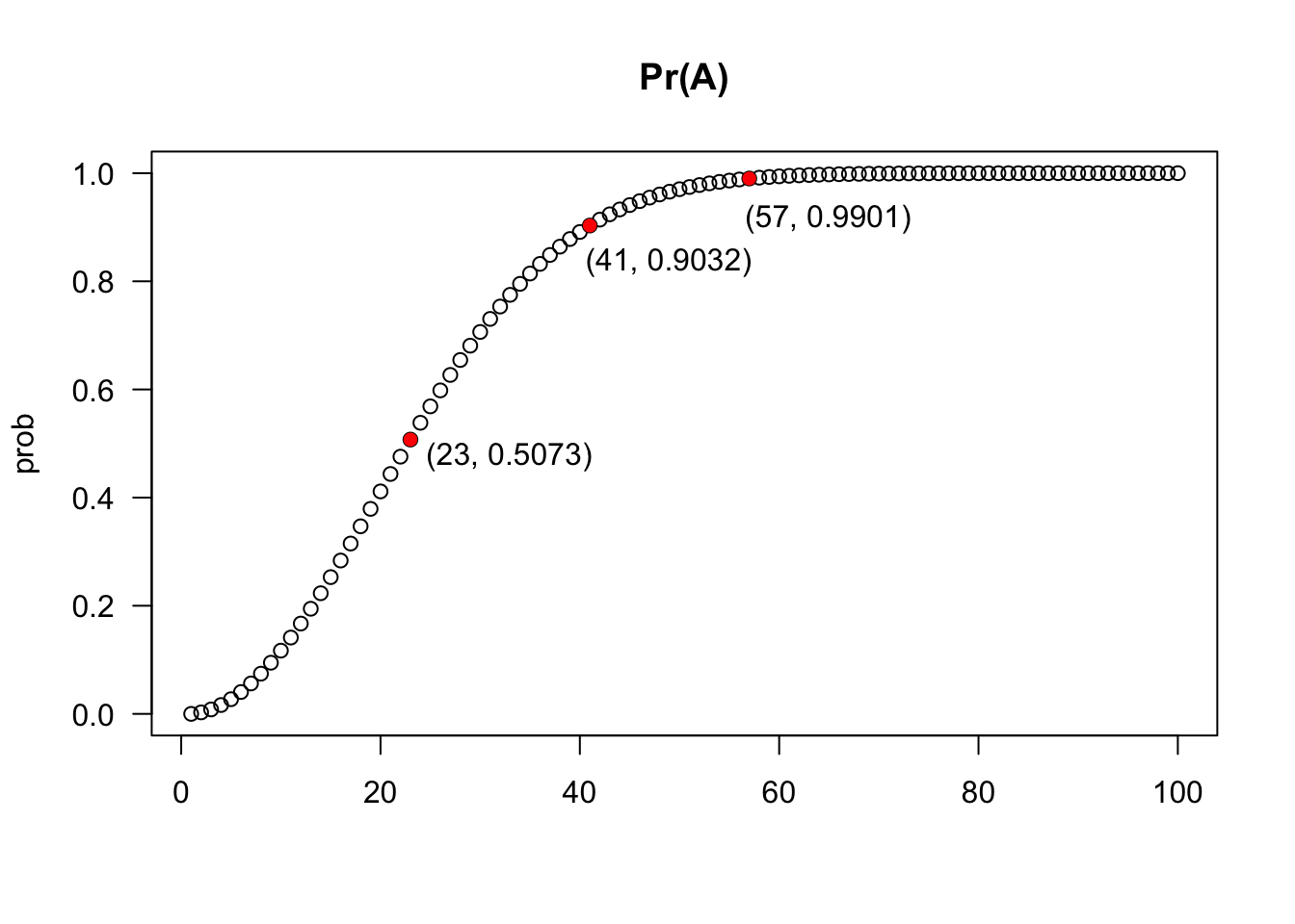
Exercise 3.7 Consider the data from Example 3.18.
a. Explain in words Eq. (3.29).
b. Show that the Equation (3.29) can be written as
\[\begin{equation}
Pr(A^c) = \left( 1 - \frac{1}{365} \right) \left(1- \frac{2}{365} \right) \cdots \left( 1- \frac{n-1}{365} \right)
\tag{3.31}
\end{equation}\]
c. Write function birthday2 implementing Eq. (3.31) and compare with birthday.
d. Watch the video https://www.youtube.com/watch?v=ofTb57aZHZs, kindly suggested by Pedro Devincenzi Ferreira.
e. For a Bayesian approach see (Diaconis and Holmes 2002).
\(\\\)