4.3 Samples
Definition 4.8 Consider the universe \(\mathcal{U} = \lbrace 1, 2, \ldots, N \rbrace\). A sample is any sequence of \(n\) units of \(\mathcal{U}\), formally denoted by \[\boldsymbol{a} = (a_1,\ldots,a_n),\] where the \(i\)-th component of \(\boldsymbol{a}\) is such that \(a_i \in \mathcal{U}\). \(\\\)
Example 4.12 Let \(\mathcal{U} = \lbrace 1, 2, 3 \rbrace\). The vectors \(\boldsymbol{a}_A = (2,3)\), \(\boldsymbol{a}_B = (3,3,1)\), \(\boldsymbol{a}_C = (2)\), \(\boldsymbol {a}_D = (2,2,3,3,1)\) are possible samples of \(\mathcal{U}\). \(\\\)
Example 4.13 In the Example 4.12, note the sample sizes \(n_A = n(\boldsymbol{a}_A) = 2\), \(n_B = n(\boldsymbol{a}_B) = 3\), \(n_C = n(\boldsymbol{a}_C) = 1\) and \(n_D = n(\boldsymbol{a}_D) = 5\).
Definition 4.9 Let \(\mathcal{A}(\mathcal{U})\) or simply \(\mathcal{A}\) be the set of all samples of \(\mathcal{U}\), of any size, and \(\mathcal{A} _{n}(\mathcal{U})\) or simply \(\mathcal{A}_{n}\) is the subclass of samples of size \(n\). \(\\\)
Example 4.14 If \(\mathcal{U} = \lbrace 1, 2, 3 \rbrace\), \[\mathcal{A}(\mathcal{U}) = \lbrace (1),(2),(3),(1,1),(1,2),(1,3),(2,1),\ldots,(3,1,2,2,1),\ldots \rbrace,\] \[\mathcal{A}_{1}(\mathcal{U}) = \lbrace (1),(2),(3) \rbrace, \] \[\mathcal{A}_{2}(\mathcal{U}) = \lbrace (1,1),(1,2),(1,3),(2,1),(2,2),(2,3),(3,1),(3,2),(3,3) \rbrace. \] Simplified \[\mathcal{A} = \lbrace 1,2,3,11,12,13,21,\ldots,31221,\ldots \rbrace,\] \[\mathcal{A}_{1} = \lbrace 1,2,3 \rbrace, \] \[\mathcal{A}_{2} = \lbrace 11,12,13,21,22,23,31,32,33 \rbrace. \]
Example 4.15 In the previous example, note the number of elements (cardinality) in each set: \[|\mathcal{U}|=3\] \[|\mathcal{A}(\mathcal{U})| = \infty\] \[|\mathcal{A}_{1}(\mathcal{U})| = 3^1 = 3\] \[|\mathcal{A}_{2}(\mathcal{U})| = 3^2 = 9\] \[\vdots\] \[|\mathcal{A}_{n}(\mathcal{U})| = |\mathcal{U}|^n.\]
4.3.1 Sampling plan
Definition 4.10 An (ordered) sampling plan is a function \(P(\boldsymbol{a})\) defined on \(\mathcal{A}(\mathcal{U})\) satisfying \[P(\boldsymbol{a}) \ge 0, \; \forall \boldsymbol{a} \in \mathcal{A}(\mathcal{U}),\] such that \[\sum_{\boldsymbol{a} \in \mathcal{A}} P(\boldsymbol{a}) = 1.\] \(\\\)
Example 4.16 Consider \(\mathcal{U} = \lbrace 1, 2, 3 \rbrace\) and \(\mathcal{A}(\mathcal{U})\) as per Example 4.14. It is possible to create infinite sample plans, such as:
Plan A \(\cdot\) Simple Random Sampling with replacement (SRSwi) \[P(11)=P(12)=P(13)=1/9 \\ P(21)=P(22)=P(23)=1/9 \\ P(31)=P(32)=P(33)=1/9 \\ P(\boldsymbol{a}) = 0, \; \forall \boldsymbol{a} \notin \mathcal{A}_{2}(\mathcal{U}).\]
Plan B \(\cdot\) Simple Random Sampling without replacement (SRSwo) \[P(12)=P(13)=1/6 \\ P(21)=P(23)=1/6 \\ P(31)=P(32)=1/6 \\ P(\boldsymbol{a}) = 0, \; \forall \boldsymbol{a} \notin \mathcal{A}_{2}(\mathcal{U}).\]
Plan C \(\cdot\) Combinations \[P(12)=P(13)=P(23)=1/3 \\ P(\boldsymbol{a}) = 0, \; \forall \boldsymbol{a} \notin \mathcal{A}_{2}(\mathcal{U}).\]
Plan D \[P(3)=9/27 \\ P(12)=P(23)=3/27 \\ P(111)=P(112)=P(113)=P(123)=1/27 \\ P(221)=P(222)=P(223)=P(231)=1/27 \\ P(331)=P(332)=P(333)=P(312)=1/27 \\ P(\boldsymbol{a}) = 0, \; \forall \boldsymbol{a} \notin \mathcal{A}(\mathcal{U}).\]
Example 4.17 Consider the sample \(\boldsymbol{a} = (1,2)\) obtained from the universe described Example 4.4 from some valid sampling plan. If subject 1 is 24 years old and 1.66m tall, and subject 2 is 32 years old and 1.81m tall, \[\boldsymbol{x} = (\boldsymbol{x}_1,\boldsymbol{x}_2) = \left( \begin{bmatrix} 24 \\ 1.66 \end{bmatrix}, \begin{bmatrix} 32 \\ 1.81 \end{bmatrix} \right) = \left( \begin{array}{cc} 24 & 32 \\ 1.66 & 1.81 \end{array} \right).\]
Definition 4.11 A statistic is a function of the sample data \(\boldsymbol{a}\) denoted by \(h(\boldsymbol{x})\), i.e., any numerical measurement calculated from the values observed in the sample. \(\\\)
Example 4.18 Consider \(\boldsymbol{x}\), the sample data matrix \(\boldsymbol{a} = (1,2)\). Examples of statistics are: \[h_1 = \frac{24+32}{2} = 28 \;\;\;\;\; \textrm{(average age)}\] \[h_2 = \frac{1.66+1.81}{2} = 1.735 \;\;\;\;\; \textrm{(average height)}\] \[h_3 = 32-24 = 8 \;\;\;\;\; \textrm{(range of ages)}\] \[h_4 = \sqrt{24^2+32^2} = \sqrt{1600} = 40 \;\;\;\;\; \textrm{(age norm)}\]
Exercise 4.4 Calculate the statistics of Example 4.18 considering the samples \(\boldsymbol{a} = (1,3)\) and \(\boldsymbol{a} = (2,3)\).
4.3.2 Sampling distributions
Definition 4.12 The sampling distribution of a statistic \(h(\boldsymbol{x})\) according to a sampling plan \(\lambda\), is the probability distribution \(H( \boldsymbol{x})\) defined over \(\mathcal{A}_\lambda\), with probability function \[p_h = P_\lambda(H(\boldsymbol{x})=h) = P(h) = \frac{f_h}{|\mathcal{A}_\lambda|}.\] \(\\\)
Example 4.19 Consider the variable age from Example 4.4 and the statistics \(h_1(\boldsymbol{x})=\frac{1}{n}\sum_{i=1}^n x_i\) and \(h_2(\boldsymbol{x})=\frac{1}{n-1}\sum_{i=1}^n (x_i-h_1(\boldsymbol{x}))^2\) applied to the sampling plan A of Example 4.16. Note that \(h_1(\boldsymbol{x})\) and \(h_2(\boldsymbol{x})\) are the sample mean and variance respectively. \(\\\)
- Plan A \(\cdot\) Simple Random Sampling with replacement (SRSwi)
| \(i\) | 1 | 2 | 3 | 4 | 5 | 6 | 7 | 8 | 9 |
| \(\boldsymbol{a}\) | 11 | 12 | 13 | 21 | 22 | 23 | 31 | 32 | 33 |
| \(P(\boldsymbol{a})\) | 1/9 | 1/9 | 1/9 | 1/9 | 1/9 | 1/9 | 1/9 | 1/9 | 1/9 |
| \(\boldsymbol{x}\) | (24,24) | (24,32) | (24,49) | (32,24) | (32,32) | (32,49) | (49,24) | (49,32) | (49,49) |
| \(h_1(\boldsymbol{x})\) | 24.0 | 28.0 | 36.5 | 28.0 | 32.0 | 40.5 | 36.5 | 40.5 | 49.0 |
| \(h_2(\boldsymbol{x})\) | 0.0 | 32.0 | 312.5 | 32.0 | 0.0 | 144.5 | 312.5 | 144.5 | 0.0 |
| \(h_1\) | 24.0 | 28.0 | 32.0 | 36.5 | 40.5 | 49.0 | Total |
| \(f_{h1}\) | 1 | 2 | 1 | 2 | 2 | 1 | 9 |
| \(p_{h1}\) | 1/9 | 2/9 | 1/9 | 2/9 | 2/9 | 1/9 | 1 |
| \(h_2\) | 0.0 | 32.0 | 144.5 | 312.5 | Total |
| \(f_{h2}\) | 3 | 2 | 2 | 2 | 9 |
| \(p_{h2}\) | 3/9 | 2/9 | 2/9 | 2/9 | 1 |
\(\\\)
Example 4.20 Consider again the variable age from Example 4.4 and the statistic \(h_1(\boldsymbol{x})=\frac{1}{n}\sum_{i=1}^n x_i\), now applied to sampling plan B of Example 4.16. \(\\\)
- Plan B \(\cdot\) Simple Random Sampling without replacement (SRSwo)
| \(i\) | 1 | 2 | 3 | 4 | 5 | 6 |
| \(\boldsymbol{a}\) | 12 | 13 | 21 | 23 | 31 | 32 |
| \(P(\boldsymbol{a})\) | 1/6 | 1/6 | 1/6 | 1/6 | 1/6 | 1/6 |
| \(\boldsymbol{x}\) | (24,32) | (24,49) | (32,24) | (32,49) | (49,24) | (49,32) |
| \(h_1(\boldsymbol{x})\) | 28.0 | 36.5 | 28.0 | 40.5 | 36.5 | 40.5 |
| \(h_1\) | 28.0 | 36.5 | 40.5 | Total |
| \(f_{h1}\) | 2 | 2 | 2 | 6 |
| \(p_{h1}\) | 2/6 | 2/6 | 2/6 | 1 |
\(\\\)
Example 4.21 Consider again the variable age from Example 4.4 and the statistic \(h_1(\boldsymbol{x})=\frac{1}{n}\sum_{i=1}^n x_i\), now applied to the sample plan C of Example 4.16. \(\\\)
- Plan C \(\cdot\) Combinations
| \(i\) | 1 | 2 | 3 |
| \(\boldsymbol{a}\) | 12 | 13 | 23 |
| \(P(\boldsymbol{a})\) | 1/3 | 1/3 | 1/3 |
| \(\boldsymbol{x}\) | (24,32) | (24,49) | (32,49) |
| \(h_1(\boldsymbol{x})\) | 28.0 | 36.5 | 40.5 |
| \(h_1\) | 28.0 | 36.5 | 40.5 | Total |
| \(f_{h1}\) | 1 | 1 | 1 | 3 |
| \(p_{h1}\) | 1/3 | 1/3 | 1/3 | 1 |
\(\\\)
Exercise 4.5 Redo the Examples 4.19, 4.20 and 4.21 considering the variable height. For the Examples 4.20 and 4.21, also calculate the statistic \(h_2(\boldsymbol{x})=\frac{1}{n-1}\sum_{i= 1}^n (x_i-h_1(\boldsymbol{x}))^2\). \(\\\)
##   Var1 Var2
## 1    1    1
## 2    2    1
## 3    3    1
## 4    1    2
## 5    2    2
## 6    3    2
## 7    1    3
## 8    2    3
## 9 3 3## [,1] [,2]
## [1,] 1 1
## [2,] 1 2
## [3,] 1 3
## [4,] 2 1
## [5,] 2 2
## [6,] 2 3
## [7,] 3 1
## [8,] 3 2
## [9,] 3 3## [,1] [,2]
## [1,] 1 2
## [2,] 1 3
## [3,] 2 1
## [4,] 2 3
## [5,] 3 1
## [6,] 3 2x1 <- c(24,32,49) # age data
n <- ncol(aasc)
# SRSwi
(xc <- cbind(x1[aasc[,1]], x1[aasc[,2]])) # age sample data with replacement## [,1] [,2]
## [1,] 24 24
## [2,] 24 32
## [3,] 24 49
## [4,] 32 24
## [5,] 32 32
## [6,] 32 49
## [7,] 49 24
## [8,] 49 32
## [9,] 49 49## [1] 24.0 28.0 36.5 28.0 32.0 40.5 36.5 40.5 49.0## mxc
## 24 28 32 36.5 40.5 49
## 1 2 1 2 2 1## mxc
## 24 28 32 36.5 40.5 49
## 1/9 2/9 1/9 2/9 2/9 1/9# vyc <- (rowMeans(xc^2)-mxc^2)*(n/(n-1))
# SRSwo
(xs <- cbind(x1[aass[,1]], x1[aass[,2]])) # age sample data without replacement## [,1] [,2]
## [1,] 24 32
## [2,] 24 49
## [3,] 32 24
## [4,] 32 49
## [5,] 49 24
## [6,] 49 32## [1] 28.0 36.5 28.0 40.5 36.5 40.5## mxs
## 28 36.5 40.5
## 2 2 2## mxs
## 28 36.5 40.5
## 1/3 1/3 1/3Example 4.23 The resolutions of Examples 4.20 and 4.21 can be implemented in the package arrangements of R. Note that samples are obtained via SRSwo through the permutations function and samples by combination, without any type of repetition, through the combinations function.
library(arrangements)
x1 <- c(24,32,49)  #age data
# SRSwi
npermutations(3,2) # number of samples via combination SRSwi
## [1] 6## [,1] [,2]
## [1,] 1 2
## [2,] 1 3
## [3,] 2 1
## [4,] 2 3
## [5,] 3 1
## [6,] 3 2## [,1] [,2]
## [1,] 24 32
## [2,] 24 49
## [3,] 32 24
## [4,] 32 49
## [5,] 49 24
## [6,] 49 32## [1] 28.0 36.5 28.0 40.5 36.5 40.5## [1] 35## [1] 3## [,1] [,2]
## [1,] 1 2
## [2,] 1 3
## [3,] 2 3## [,1] [,2]
## [1,] 24 32
## [2,] 24 49
## [3,] 32 49## [1] 28.0 36.5 40.5## [1] 35Exercise 4.6 Generalize the Examples 4.22 and 4.21 for any sample size, parameterizing the options with and without replacement, as well as for combinations. Finally, add an argument that allows you to calculate any statistic.
Central Limit Theorem
The Central Limit Theorem (CLT) is one of the main results of Probability. It shows that, under certain conditions reasonably achieved in practice, the sum or average of a sequence of independent and identically distributed random variables (iid)21 are approximately normally distributed. This result allows the approximate resolution of problems that involve many calculations, usually impractical given the volume of operations required.
Theorem 4.1 (Lindeberg-Lévy Central Limit Theorem) Let \(X_{1}, X_{2}, \ldots, X_{n}\) be a sequence of iid random variables with \(E(X_{i}) = \mu\) and \(V(X_{i}) = \sigma^2\). Considering \(S=X_{1}+X_{2}+\ldots+X_{n}\), \(M=S/n\) and if \(n \longrightarrow \infty\), then \[\begin{equation} Z = \frac{S - n\mu}{\sigma \sqrt{n}} = \dfrac{M - \mu}{\sigma / \sqrt{n}} \xrightarrow{D} \mathcal{N}(0,1). \tag{4.4} \end{equation}\]
Continuity correction occurs when 0.5 is added to the numerator of Equation (4.4). (James 2010) points out that central is the theorem, not the limit. The origin of the expression is attributed to the Hungarian mathematician George Pólya, when referring to der zentrale Grenzwertsatz, i.e., the ‘central’ refers to the ‘limit theorem’.
Proportion sampling distribution
The proportion is an average in the case where the variable only accepts the values 0 and 1, therefore the CLT applies directly to this type of structure.
Example 4.24 (Approximation of the binomial by the normal) If we consider \(n=420\) flips of a coin with \(p=0.5\), we have that the v.a. \(X\): number of heads is such that \(X \sim \mathcal{B} (420.0.5)\). The probability of getting up to 200 heads can be approximated using the CLT. \[ Pr(X \le 200) \approx Pr \left( Z < \dfrac{200-420\times 0.5}{\sqrt{420 \times 0.5 \times 0.5}} \right) = \Phi(-0.9759) \approx 0.164557. \] Using continuity correction, \[ Pr(X \le 200) \approx Pr \left( Z < \dfrac{200+0.5-420\times 0.5}{\sqrt{420 \times 0.5 \times 0.5}} \right ) = \Phi(-0.9271) \approx 0.176936. \] With a computer it is possible to calculate the exact probability, notice how close the results are. \[ Pr(X \le 200) = \left[ {420 \choose 0} + {420 \choose 1} + \cdots + {420 \choose 200} \right] 0.5^{420} = 0.1769429. \]
n <- 420
p <- 0.5
S <- 200
mS <- n*p  # 210
sS <- sqrt(n*p*(1-p))  # 10.24695
# Approximation of the binomial by the normal WITHOUT continuity correction
(z <- (S-mS)/sS)
## [1] -0.9759001## [1] 0.164557## [1] -0.9271051## [1] 0.176936## [1] 0.1769429Sampling distribution of the mean
Based on the Central Limit Theorem, it is known that the distribution of sample means of any variable \(X\) that satisfies the conditions of the theorem converges to the normal distribution. Consider that \(X\) has any distribution \(\mathcal{D}\), with mean \(\mu\) and standard deviation \(\sigma\), symbolized by \[X \sim \mathcal{D}(\mu,\sigma) .\] By CLT, the distribution of sample means of any size \(n_0\) is such that \[\bar{X}_{n_0} \sim \mathcal{N} \left( \mu,\frac{\sigma} {\sqrt{n_0}} \right).\] The measurement \(\sigma/\sqrt{n_0}\) is known as standard error (of the mean) (SEM). The CLT is an asymptotic result22, so the closer \(\mathcal{D}\) is to \(\mathcal{N}\), the faster the convergence of \(\bar{X}_{n_0}\) must be for normal distribution.
Example 4.25 Consider the random variable \(X\): IQ of the world population, assumed with a normal distribution of mean \(\mu=100\) and standard deviation of \(\sigma=15\), noted by \(X \sim \mathcal{N}(100.15)\).
mu <- 100 # X average
sigma <- 15  # X standard deviation
curve(dnorm(x, mean=mu, sd=sigma), from=mu-3*sigma, to=mu+3*sigma) # X ~ N(100,15)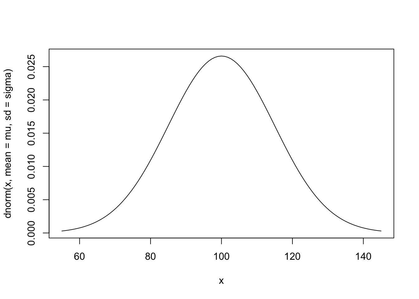
n0 <- 25 # sample size
n <- 200 # number of samples
set.seed(1234) # fixing pseudo-random seed to ensure replication
a <- MASS::mvrnorm(n0, mu = rep(mu,n), Sigma = sigma^2*diag(n)) # samples
ma <- colMeans(a) # means of n samples
hist(ma) # histogram of averages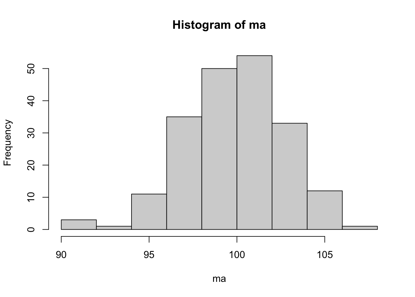
## [1] 99.90468## [1] 2.817847## [1] 3Exercise 4.7 Redo the Example 4.25 changing the values of n0 and n, checking what happens in the histogram, mean and standard deviation of ma. Pay attention to the fact that values of n greater than 1000 can make the process computationally expensive.
4.3.3 Representative sample
We often hear the argument that a good sample is one that is representative. When asked about the definition of a representative sample, the most common answer is something like: “one that is a micro representation of the universe”. But to be sure that a sample is a micro representation of the universe for a given characteristic of interest, one must know the behavior of that same characteristic of the population. Then, the population’s knowledge would be so great that sample collection would become unnecessary.
(Bolfarine and Bussab 2005, 14)
In this material the term “representative” will be conditional. For example, “representative considering the approximate population proportions of the variables \(X_1, \ldots, X_n\)”.
4.3.4 Sample types
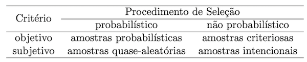
Objective probabilistic procedures are better accepted academically, even though they cannot always be implemented in practice. When this occurs, procedures that are possible to be carried out can be considered.