5.9 Teste de Hipóteses
Seja um parâmetro \(\theta\) pertencente a um espaço paramétrico \(\Theta\), i.e., o conjunto de todos os possíveis valores de \(\theta\). Considere uma partição tal que \(\Theta_0 \cup \Theta_1 = \Theta\) e \(\Theta_0 \cap \Theta_1 = \emptyset\). Um teste de hipóteses é uma regra de decisão que permite decidir, à luz das informações disponíveis, se é mais verossímil admitir \(\theta \in \Theta_0\) ou \(\theta \in \Theta_1\).
Figura 5.2: Did the sun just explode? de https://xkcd.com/1132/
Exercício 5.27 Veja
- Seção 3.4 de (Paulino et al. 2003).
- Capítulo 9 de (Press 2003).
Exercício 5.28 Verifique a hipótese de que a palavra ‘hipótese’ vem do grego hipo (fraca) + tese = ‘tese fraca’ conforme sugerido por Renato Janine Ribeiro no Provoca de 24/08/2021.
5.9.1 Fator de Bayes
In a 1935 paper and in his book Theory of Probability, Jeffreys developed a methodology for quantifying the evidence in favor of a scientific theory. The centerpiece was a number, now called the Bayes factor, which is the posterior odds of the null hypothesis when the prior probability on the null is one-half. (Kass and Raftery 1995, 773)
Suponha que deseja-se testar \(H_0: \theta \in \Theta_0\) vs \(H_1:\theta \in \Theta_1\). Do teorema de Bayes obtém-se
\[\begin{equation} P(H_i|D) = \frac{P(D|H_i)P(H_i)}{P(D|H_0)P(H_0) + P(D|H_1)P(H_1)} \tag{5.14} \end{equation}\]
Desta forma
\[\begin{equation} \frac{P(H_1|D)}{P(H_0|D)} = \frac{P(D|H_1)}{P(D|H_0)} \frac{P(H_1)}{P(H_0)} \nonumber \tag{5.15} \end{equation}\]
Aplicando \(P(H_0)=P(H_1)=1/2\) conforme (Jeffreys 1935) e (Jeffreys 1961), define-se o fator de Bayes por
\[\begin{equation} B_{10} = \frac{P(D|H_1)}{P(D|H_0)} \tag{5.16} \end{equation}\]
Conforme (Kass and Raftery 1995, 776), no caso mais simples, quando as duas hipóteses são distribuições únicas sem parâmetros livres (o caso do teste “simples versus simples”), \(B_{10}\) é a razão de verossimilhança. Em outros casos, quando há parâmetros desconhecidos sob uma ou ambas as hipóteses, o fator de Bayes ainda é dado por (5.14), mas as densidades \(P(D|H_0)\) e \(P(D|H_1)\) são obtidas integrando, e não maximizando sobre o espaço de parâmetros.
Podem-se considerar as referências sugeridas por (Kass and Raftery 1995, 777).
| \(2 \log_e B_{10}\) | \(B_{10}\) | Evidência contra \(H_0\) |
|---|---|---|
| 0 a 2 | 1 a 3 | Nem vale mencionar |
| 2 a 6 | 3 a 20 | Positiva |
| 6 a 10 | 20 a 150 | Forte |
| >10 | >150 | Muito forte |
5.9.1.1 Pacote BayesFactor
(Morey and Rouder 2024) apresentam o pacote BayesFactor.
Exemplo 5.35 Podemos comparar as funções clássicas com BayesFactor::ttestBF(). De acordo com a documentação, “o fator de Bayes fornecido por ttestBF testa a hipótese nula de que a média (ou diferença média) de uma população normal é \(\mu_0\)”.
As hipóteses podem ser escritas da seguinte forma: \[\left\{ \begin{array}{l} H_0: y_i \sim N(\mu_0,\sigma^2) \\ H_1: y_i \sim N(\mu_1,\sigma^2) \\ \end{array} \right. \]
Conforme apontado por Morey and Rouder (2011),409, Jeffreys (1961) sugere colocar prioris no tamanho do efeito padronizado (\(\delta=\mu/\sigma\)). Neste caso, \(y_i \sim N(\sigma\delta,\sigma^2)\). Os autores ainda indicam que “essa estrutura a priori é inspirada pelo conhecimento de que os tamanhos reais dos efeitos normalmente não são grandes, e que o analista é agnóstico quanto à direção de qualquer efeito possível”. Apontam ainda que a priori com distribuição Cauchy padrão para \(\delta\) “quantifica uma suposição de que parâmetros verdadeiros excessivamente grandes são muito menos plausíveis do que tamanhos de efeito pequenos, mas ainda são possíveis”.
A estrutura da priori para \(\delta\) é expressa da seguinte forma. \[\left\{ \begin{array}{l} H_0: \delta = 0\\ H_1: \delta \sim Cauchy(r) \\ \end{array} \right. \]
A priori não informativa imprópria (de Jeffreys) para \(\sigma^2\) é dada por
\[\begin{equation} \pi(\sigma^2) \propto \frac{1}{\sigma^2}. \tag{5.1} \end{equation}\]
A combinação destas prioris para \(\delta\) e \(\sigma^2\) é chamada priori de Jeffreys–Zellner–Siow (JZS).
| Parâmetro de escala | Valor de \(r\) |
|---|---|
| Medium (padrão) | \(\frac{\sqrt{2}}{2}\) |
| Wide | \(1\) (Cauchy padrão ou \(t_1\)) |
| Ultrawide | \(\sqrt{2}\) |
O fator de Bayes é calculado via quadratura gaussiana, para mais detalhes veja a Rouder et al. (2009), Morey et al. (2011) e Morey and Rouder (2011).
## classical paired t test
t.test(x = sleep2$extra[sleep2$group==1],
       y = sleep2$extra[sleep2$group==2], paired = TRUE)
##
## Paired t-test
##
## data: sleep2$extra[sleep2$group == 1] and sleep2$extra[sleep2$group == 2]
## t = -4.0621, df = 9, p-value = 0.002833
## alternative hypothesis: true mean difference is not equal to 0
## 95 percent confidence interval:
## -2.4598858 -0.7001142
## sample estimates:
## mean difference
## -1.58# classical Wilcoxon (signed rank test (median = 0 versus median > 0)
wilcox.test(x = sleep2$extra[sleep2$group==1],
y = sleep2$extra[sleep2$group==2], paired = TRUE)##
## Wilcoxon signed rank exact test
##
## data: sleep2$extra[sleep2$group == 1] and sleep2$extra[sleep2$group == 2]
## V = 0, p-value = 0.003906
## alternative hypothesis: true location shift is not equal to 0## bayesian paired t test
ttestBF(x = sleep2$extra[sleep2$group == 1],
y = sleep2$extra[sleep2$group == 2], paired = TRUE)## Bayes factor analysis
## --------------
## [1] Alt., r=0.707 : 17.25888 ±0%
##
## Against denominator:
## Null, mu = 0
## ---
## Bayes factor type: BFoneSample, JZSExemplo 5.36 Em Python.
import matplotlib.pyplot as plt
import pandas as pd
from scipy.stats import ttest_rel, wilcoxon
from bayesfactor import ttestBF
# Carregando os dados do conjunto de dados sleep
sleep2 = pd.DataFrame({
'extra':[0.7,-1.6,-0.2,-1.2,-0.1,3.4,3.7,0.8,0.0,2.0,1.9,0.8,1.1,0.1,-0.1,4.4,5.5,1.6,4.6,3.4],
'group':[1,1,1,1,1,1,1,1,1,1,2,2,2,2,2,2,2,2,2,2],
'ID':[1,2,3,4,5,6,7,8,9,10,1,2,3,4,5,6,7,8,9,10]
})
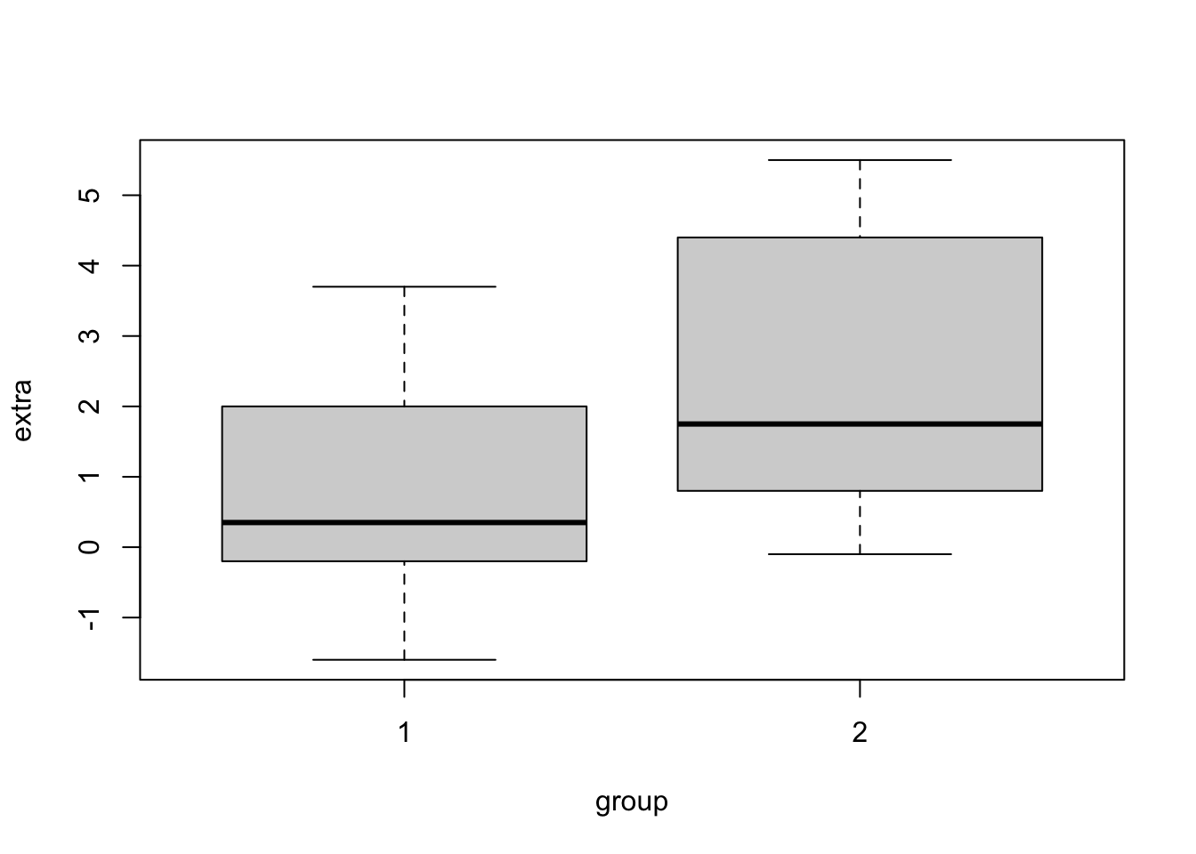
# Gráfico de dispersão
plt.figure(figsize=(8, 6))
plt.scatter(sleep2['group'], sleep2['extra'])
plt.xlabel('Grupo', fontsize=12)
plt.ylabel('Diferença', fontsize=12)
plt.title('Diferença de horas de sono por grupo', fontsize=16)
plt.xticks([1, 2])
plt.show()
# Teste t pareado clássico
t_stat, p_value = ttest_rel(sleep2['extra'][sleep2['group'] == 1],
sleep2['extra'][sleep2['group'] == 2])
print(f"Teste t pareado clássico: t={t_stat:.4f},p={p_value:.4f}")
# Teste de Wilcoxon (teste de postos sinalizados) clássico
w_stat, p_value = wilcoxon(sleep2['extra'][sleep2['group'] == 1],
sleep2['extra'][sleep2['group'] == 2])
print(f"Teste de Wilcoxon clássico: w={w_stat:.4f},p={p_value:.4f}")
# Teste t pareado bayesiano
bf = ttestBF(x=sleep2['extra'][sleep2['group'] == 1],
y=sleep2['extra'][sleep2['group'] == 2], paired=True)
print(f"Fator de Bayes para o teste t pareado: {bf:.4f}")Exercício 5.29
Exemplo 5.37 Exemplo Moon and Agression de (Moore and McCabe 1989, 410), que fornece o número de comportamentos agressivos de pacientes com demência durante duas fases do ciclo lunar (cheia e não-cheia). Cada linha corresponde a um participante.
# lendo dados
ma <- read.csv('https://filipezabala.com/data/moon-aggression.csv')

# gráfico
boxplot(ma)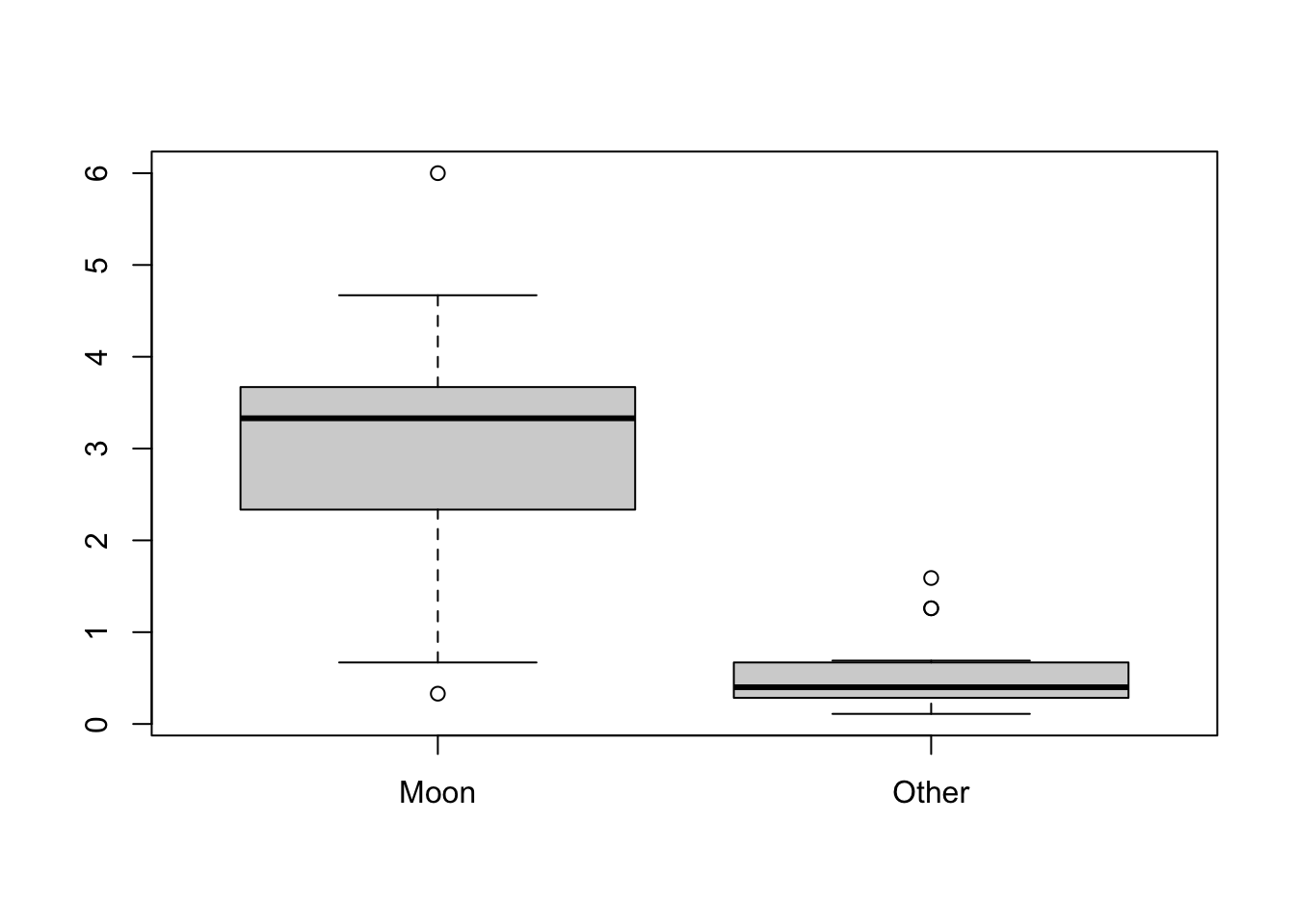
##
##  Paired t-test
##
## data:  ma$Moon and ma$Other
## t = 6.4518, df = 14, p-value = 1.518e-05
## alternative hypothesis: true mean difference is not equal to 0
## 95 percent confidence interval:
##  1.623968 3.241365
## sample estimates:
## mean difference
##        2.432667
# classical Wilcoxon signed rank test (median=0 versus median>0)
wilcox.test(x = ma$Moon,
y = ma$Other, paired = TRUE)##
## Wilcoxon signed rank exact test
##
## data: ma$Moon and ma$Other
## V = 119, p-value = 0.0001221
## alternative hypothesis: true location shift is not equal to 0## Bayes factor analysis
## --------------
## [1] Alt., r=0.707 : 1521.194 ±0%
##
## Against denominator:
## Null, mu = 0
## ---
## Bayes factor type: BFoneSample, JZSExemplo 5.38 Em Python.
import matplotlib.pyplot as plt
import pandas as pd
from scipy.stats import ttest_rel, wilcoxon
from bayesfactor import ttestBF

# Lendo os dados
ma = pd.read_csv('https://filipezabala.com/data/moon-aggression.csv')

# Gráfico de boxplot
ma.boxplot()
plt.title('Agressividade na Lua vs Outros Dias')
plt.ylabel('Nível de Agressividade')
plt.show()

# Teste t pareado clássico
t_stat, p_value = ttest_rel(ma['Moon'], ma['Other'])
print(f"Teste t pareado clássico: t={t_stat:.4f},p={p_value:.4f}")

# Teste de Wilcoxon (teste de postos sinalizados) clássico
w_stat, p_value = wilcoxon(ma['Moon'], ma['Other'])
print(f"Teste de Wilcoxon clássico: w={w_stat:.4f},p={p_value:.4f}")

# Teste t pareado bayesiano
bf = ttestBF(x=ma['Moon'], y=ma['Other'], paired=True)
print(f"Fator de Bayes para o teste t pareado: {bf:.4f}")
Exercício 5.31 Veja
- (Kass and Raftery 1995)
- Seção 3.4.1 de (Paulino et al. 2003)
- Seção 9.5.1 de (Press 2003)
- A vinheta de
BFpack(Mulder et al. 2021) em https://cran.r-project.org/package=BFpack.
5.9.2 FBST
FBST é o acrônimo para Full Bayesian Significance Test, proposto por (Pereira and Stern 1999) para testar hipóteses precisas (sharp hypotheses), amplamente revisado em (Pereira et al. 2008) e (Pereira and Stern 2020). Para idéias iniciais, veja o artigo de Eduardo E. R. Junior (2016-04-20).
5.9.2.1 Pacote fbst
Kelter (2022) apresenta fbst, um pacote R para o Full Bayesian Significance Test para testar uma hipótese nula precisa contra sua alternativa por meio do valor de evidência \(e\) conforme (Pereira and Stern 1999).
# https://cran.r-project.org/package=fbst
library(fbst)

set.seed(57)
grp1 <- rnorm(50,0,1.5)
grp2 <- rnorm(50,0.8,3.2)

p <- as.vector(BayesFactor::ttestBF(x=grp1,y=grp2,
                                    posterior = TRUE,
                                    iterations = 3000,
                                    rscale = "medium")[,4])

# flat reference function
res <- fbst(posteriorDensityDraws = p, nullHypothesisValue = 0,
            dimensionTheta = 2, dimensionNullset = 1)
summary(res)
## Full Bayesian Significance Test for testing a sharp hypothesis against its alternative:
## Reference function: Flat
## Hypothesis H_0:Parameter= 0 against its alternative H_1
## Bayesian e-value against H_0: 0.9265912
## Standardized e-value: 0.02228466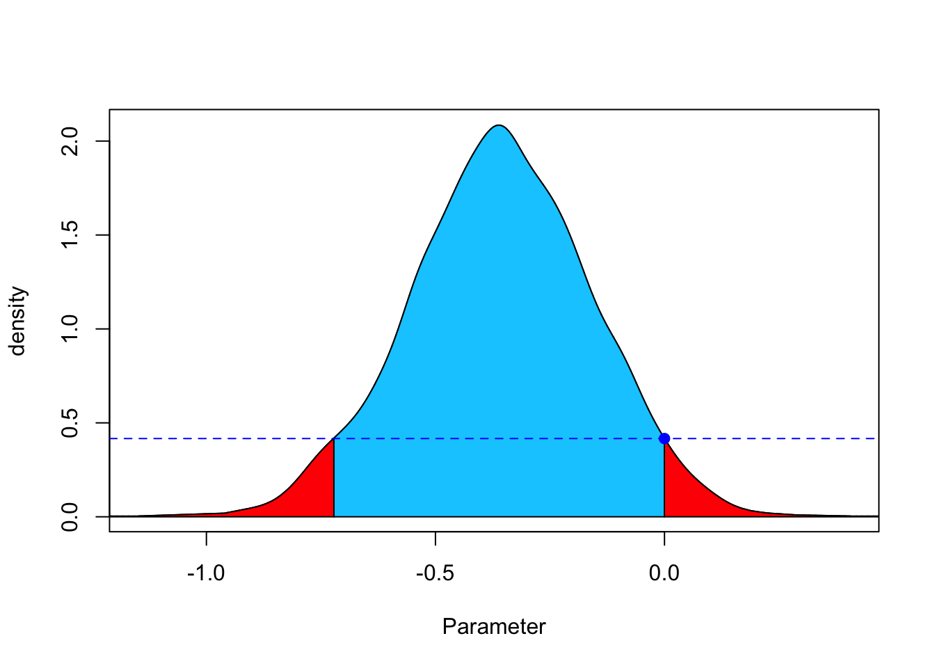
# medium Cauchy C(0,1) reference function
res_med <- fbst(posteriorDensityDraws = p, nullHypothesisValue = 0,
                dimensionTheta = 2, dimensionNullset = 1, FUN = dcauchy,
                par = list(location = 0, scale = sqrt(2)/2))
summary(res_med)
## Full Bayesian Significance Test for testing a sharp hypothesis against its alternative:
## Reference function: User-defined
## Hypothesis H_0:Parameter= 0 against its alternative H_1
## Bayesian e-value against H_0: 0.9529035
## Standardized e-value: 0.01343346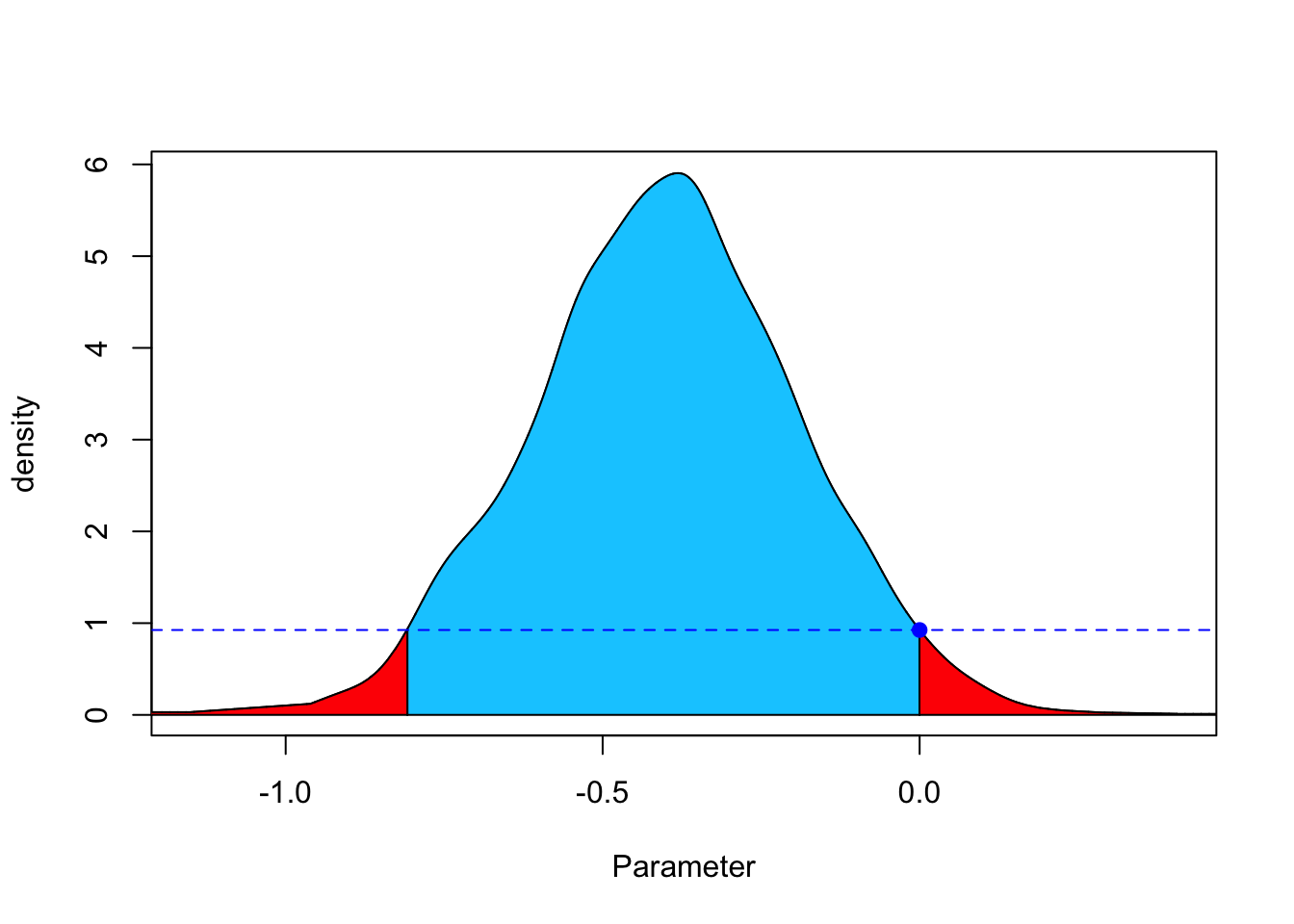
5.9.3 Valores-p bayesiano
O valor-p preditivo a posteriori (Paulino et al. 2003) e a probabilidade de direção (Makowski et al. 2019) são reportados na literatura como ‘valores-p bayesianos’.
5.9.4 Combinando ferramentas
(Gannon et al. 2019) sugerem que “os pesquisadores não precisam abandonar completamente o valor p, o índice de significância mais conhecido, mas devem parar de usar níveis de significância que não dependem do tamanho da amostra”.
tab <- matrix(c(1,7, 4,4), nrow = 2, byrow = TRUE)
rownames(tab) <- c('C','T') # Controle/Tratamento
colnames(tab) <- c('+','-') # Respondeu positivamente/negativamente
(tab <- as.table(tab))
## + -
## C 1 7
## T 4 4##
## Pearson's Chi-squared test
##
## data: tab
## X-squared = 2.6182, df = 1, p-value = 0.1056##
## Pearson's Chi-squared test with Yates' continuity correction
##
## data: tab
## X-squared = 1.1636, df = 1, p-value = 0.2807##
## Fisher's Exact Test for Count Data
##
## data: tab
## p-value = 0.2821
## alternative hypothesis: true odds ratio is not equal to 1
## 95 percent confidence interval:
## 0.002553456 2.416009239
## sample estimates:
## odds ratio
## 0.1624254# Fator de Bayes
fh <- function(x,y){
(choose(8,x)*choose(8,y))/(17*choose(16,x+y))
}
fa <- 1/81
bf <- function(x,y){
fh(x,y)/fa
}
BF <- matrix(nrow = 9, ncol = 9)
rownames(BF) <- paste0('x.',0:8)
colnames(BF) <- paste0('y.',0:8)
for(i in 0:8){
for(j in 0:8){
BF[i+1,j+1] <- bf(j,i)
}
}
addmargins(round(BF,3)) # note a questão do arredondamento## y.0 y.1 y.2 y.3 y.4 y.5 y.6 y.7 y.8 Sum
## x.0 4.765 2.382 1.112 0.476 0.183 0.061 0.017 0.003 0.000 8.999
## x.1 2.382 2.541 1.906 1.173 0.611 0.267 0.093 0.024 0.003 9.000
## x.2 1.112 1.906 2.052 1.710 1.166 0.653 0.290 0.093 0.017 8.999
## x.3 0.476 1.173 1.710 1.866 1.633 1.161 0.653 0.267 0.061 9.000
## x.4 0.183 0.611 1.166 1.633 1.814 1.633 1.166 0.611 0.183 9.000
## x.5 0.061 0.267 0.653 1.161 1.633 1.866 1.710 1.173 0.476 9.000
## x.6 0.017 0.093 0.290 0.653 1.166 1.710 2.052 1.906 1.112 8.999
## x.7 0.003 0.024 0.093 0.267 0.611 1.173 1.906 2.541 2.382 9.000
## x.8 0.000 0.003 0.017 0.061 0.183 0.476 1.112 2.382 4.765 8.999
## Sum 8.999 9.000 8.999 9.000 9.000 9.000 8.999 9.000 8.999 80.996## [1] 0.6108597## [1] 0.09228027Exemplo 5.39 Em Python.
import numpy as np
from scipy.stats import chi2_contingency, fisher_exact
from scipy.special import comb

# Criando a tabela de contingência
tab = np.array([[1, 7], [4, 4]])

# Teste qui-quadrado sem correção de Yates
chi2_stat, p_value, dof, expected = chi2_contingency(tab, correction=False)
print(f"Teste qui-quadrado sem correção: chi2={chi2_stat:.4f},p={p_value:.4f},dof={dof}")

# Teste qui-quadrado com correção de Yates
chi2_stat, p_value, dof, expected = chi2_contingency(tab, correction=True)
print(f"Teste qui-quadrado com correção: chi2={chi2_stat:.4f},p={p_value:.4f},dof={dof}")

# Teste exato de Fisher
odds_ratio, p_value = fisher_exact(tab)
print(f"Teste exato de Fisher: odds ratio={odds_ratio:.4f},p={p_value:.4f}")

# Fator de Bayes
def fh(x, y):
    return (comb(8, x) * comb(8, y)) / (17 * comb(16, x + y))

fa = 1/81

def bf(x, y):
    return fh(x, y) / fa

BF = np.zeros((9, 9))
for i in range(9):
    for j in range(9):
        BF[i, j] = bf(j, i)

# Adicionando margens à matriz BF (aproximado)
BF_with_margins = np.c_[BF, np.sum(BF, axis=1)]
BF_with_margins = np.r_[BF_with_margins,[np.sum(BF_with_margins,axis=0)]]
print("\nMatriz BF com margens (aproximada):")
print(np.round(BF_with_margins, 3))

# Calculando o BF observado
BF_obs = bf(1, 4)
print(f"\nBF observado: {BF_obs:.4f}")

# Calculando o p-value (aproximado)
p_value_bf = np.sum(BF[BF <= BF_obs]) / 81
print(f"P-value (aproximado): {p_value_bf:.4f}")
5.9.5 Testes agnósticos
[A]gnostic tests, in which one can accept, reject or remain agnostic with respect to a given hypothesis. (Stern 2016, 1)
References
https://stats.stackexchange.com/questions/570605/understanding-the-jeffreys-zellner-siow-jzs-prior-in-bayesian-t-tests↩︎
https://pingouin-stats.org/build/html/generated/pingouin.bayesfactor_ttest.html#pingouin.bayesfactor_ttest↩︎
https://terrytao.wordpress.com/2024/08/02/what-are-the-odds-ii-the-venezuelan-presidential-election/↩︎