5.10 Teste de Hipóteses

• Seção 3.4 de (Paulino, Turkman, and Murteira 2003)
  
• Capítulo 9 de (S. J. Press 2003)

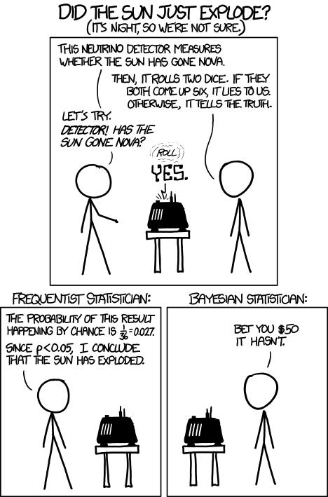
“Did the sun just explode?” by xkcd.com

5.10.1 Fator de Bayes

• (Kass and Raftery 1995)
  
• Seção 3.4.1 de (Paulino, Turkman, and Murteira 2003)
  
• Seção 9.5.1 de (S. J. Press 2003)

5.10.1.1 Pacote BayesFactor

(Morey and Rouder 2022) apresentam o pacote BayesFactor.

library(BayesFactor)
BFManual()

Exemplo 5.13 Exemplo da documentação.

## Sleep data from t test example
sleep2 <- datasets::sleep
plot(extra ~ group, data = sleep2)

## classical paired t test
t.test(x = sleep2$extra[sleep2$group==1], 
       y = sleep2$extra[sleep2$group==2], paired = TRUE)

## 
##  Paired t-test
## 
## data:  sleep2$extra[sleep2$group == 1] and sleep2$extra[sleep2$group == 2]
## t = -4.0621, df = 9, p-value = 0.002833
## alternative hypothesis: true mean difference is not equal to 0
## 95 percent confidence interval:
##  -2.4598858 -0.7001142
## sample estimates:
## mean difference 
##           -1.58

# classical Wilcoxon (signed rank test (median = 0 versus median > 0)
wilcox.test(x = sleep2$extra[sleep2$group==1], 
            y = sleep2$extra[sleep2$group==2], paired = TRUE)

## 
##  Wilcoxon signed rank test with continuity correction
## 
## data:  sleep2$extra[sleep2$group == 1] and sleep2$extra[sleep2$group == 2]
## V = 0, p-value = 0.009091
## alternative hypothesis: true location shift is not equal to 0

## bayesian paired t test
ttestBF(x = sleep2$extra[sleep2$group == 1], 
        y = sleep2$extra[sleep2$group == 2], paired = TRUE)

## Bayes factor analysis
## --------------
## [1] Alt., r=0.707 : 17.25888 ±0%
## 
## Against denominator:
##   Null, mu = 0 
## ---
## Bayes factor type: BFoneSample, JZS

Exercício 5.8 Veja a documentação de pingouin.bayesfactor_ttest no link a seguir.
https://pingouin-stats.org/build/html/generated/pingouin.bayesfactor_ttest.html#pingouin.bayesfactor_ttest

Exemplo 5.14 Exemplo Moon and Agression.

# lendo dados
ma <- read.csv('https://filipezabala.com/data/moon-aggression.csv')

# gráfico
boxplot(ma)

## classical paired t test
t.test(x = ma$Moon, 
       y = ma$Other, paired = TRUE)

## 
##  Paired t-test
## 
## data:  ma$Moon and ma$Other
## t = 6.4518, df = 14, p-value = 1.518e-05
## alternative hypothesis: true mean difference is not equal to 0
## 95 percent confidence interval:
##  1.623968 3.241365
## sample estimates:
## mean difference 
##        2.432667

# classical Wilcoxon (signed rank test (median = 0 versus median > 0)
wilcox.test(x = ma$Moon, 
            y = ma$Other, paired = TRUE)

## 
##  Wilcoxon signed rank exact test
## 
## data:  ma$Moon and ma$Other
## V = 119, p-value = 0.0001221
## alternative hypothesis: true location shift is not equal to 0

## bayesian paired t test
ttestBF(x = ma$Moon, 
        y = ma$Other, paired = TRUE)

## Bayes factor analysis
## --------------
## [1] Alt., r=0.707 : 1521.194 ±0%
## 
## Against denominator:
##   Null, mu = 0 
## ---
## Bayes factor type: BFoneSample, JZS

5.10.1.2 Pacote BFpack

(Mulder et al. 2021) apresentam o pacote BFpack.

Exercício 5.9 Veja a vinheta de BFpack em https://cran.r-project.org/package=BFpack.

5.10.2 FBST

FBST é o acrônimo para Full Bayesian Significance Test.
- Proposta de (Carlos Alberto de Bragança Pereira and Stern 1999) para testar hipóteses precisas (sharp hypotheses)
- Amplamente revisado em (Carlos A. de Bragança Pereira et al. 2008) e (Carlos Alberto de B. Pereira and Stern 2020)
- https://jreduardo.github.io/ce227-bayes/04-fbst.html

5.10.2.1 Pacote fbst

(Kelter 2020) apresenta o pacote de R fbst.

# https://cran.r-project.org/package=fbst
library(fbst)

set.seed(57)
grp1 <- rnorm(50,0,1.5)
grp2 <- rnorm(50,0.8,3.2)

p <- as.vector(BayesFactor::ttestBF(x=grp1,y=grp2, 
                                    posterior = TRUE, iterations = 3000, 
                                    rscale = "medium")[,4])

# flat reference function
res <- fbst(posteriorDensityDraws = p, nullHypothesisValue = 0, 
            dimensionTheta = 2, dimensionNullset = 1)
summary(res)

## Full Bayesian Significance Test for testing a sharp hypothesis against its alternative:
## Reference function: Flat 
## Hypothesis H_0:Parameter= 0 against its alternative H_1
## Bayesian e-value against H_0: 0.92749 
## Standardized e-value: 0.02197123

plot(res)

# medium Cauchy C(0,1) reference function
res_med <- fbst(posteriorDensityDraws = p, nullHypothesisValue = 0, 
                dimensionTheta = 2, dimensionNullset = 1, FUN = dcauchy, 
                par = list(location = 0, scale = sqrt(2)/2))
summary(res_med)

## Full Bayesian Significance Test for testing a sharp hypothesis against its alternative:
## Reference function: User-defined 
## Hypothesis H_0:Parameter= 0 against its alternative H_1
## Bayesian e-value against H_0: 0.9538276 
## Standardized e-value: 0.01313566

plot(res_med)

5.10.3 Valores-p bayesiano

O valor-p preditivo a posteriori (Paulino, Turkman, and Murteira 2003) e a probabilidade de direção (Makowski et al. 2019) são reportados na literatura como ‘valores-pr bayesianos’.

5.10.4 Combinando ferramentas

(Gannon, Pereira, and Polpo 2019)

5.10.4.1 Comparando proporções

The observed results in this example are that only one of the patients in the control arm responded positively, but in the case arm there were four positive outcomes. (Gannon, Pereira, and Polpo 2019, 217)

tab <- matrix(c(1,7, 4,4), nrow = 2, byrow = TRUE)
rownames(tab) <- c('C', 'T') # Controle/Tratamento
colnames(tab) <- c('+', '-') # Respondeu positivamente/negativamente
(tab <- as.table(tab))

##   + -
## C 1 7
## T 4 4

# Teste qui-quadrado sem correção de Yates
chisq.test(tab, correct = FALSE)

## 
##  Pearson's Chi-squared test
## 
## data:  tab
## X-squared = 2.6182, df = 1, p-value = 0.1056

# Teste qui-quadrado com correção de Yates
chisq.test(tab)

## 
##  Pearson's Chi-squared test with Yates' continuity correction
## 
## data:  tab
## X-squared = 1.1636, df = 1, p-value = 0.2807

# Teste exato de Fisher
fisher.test(tab)

## 
##  Fisher's Exact Test for Count Data
## 
## data:  tab
## p-value = 0.2821
## alternative hypothesis: true odds ratio is not equal to 1
## 95 percent confidence interval:
##  0.002553456 2.416009239
## sample estimates:
## odds ratio 
##  0.1624254

# Fator de Bayes
fh <- function(x,y){
  (choose(8,x)*choose(8,y))/(17*choose(16,x+y))
}
fa <- 1/81
bf <- function(x,y){
  fh(x,y)/fa
}
BF <- matrix(nrow = 9, ncol = 9)
rownames(BF) <- paste0('x.',0:8)
colnames(BF) <- paste0('y.',0:8)
for(i in 0:8){
  for(j in 0:8){
    BF[i+1,j+1] <- bf(j,i)
  }
}
addmargins(round(BF,3)) # note a questão do arredondamento

##       y.0   y.1   y.2   y.3   y.4   y.5   y.6   y.7   y.8    Sum
## x.0 4.765 2.382 1.112 0.476 0.183 0.061 0.017 0.003 0.000  8.999
## x.1 2.382 2.541 1.906 1.173 0.611 0.267 0.093 0.024 0.003  9.000
## x.2 1.112 1.906 2.052 1.710 1.166 0.653 0.290 0.093 0.017  8.999
## x.3 0.476 1.173 1.710 1.866 1.633 1.161 0.653 0.267 0.061  9.000
## x.4 0.183 0.611 1.166 1.633 1.814 1.633 1.166 0.611 0.183  9.000
## x.5 0.061 0.267 0.653 1.161 1.633 1.866 1.710 1.173 0.476  9.000
## x.6 0.017 0.093 0.290 0.653 1.166 1.710 2.052 1.906 1.112  8.999
## x.7 0.003 0.024 0.093 0.267 0.611 1.173 1.906 2.541 2.382  9.000
## x.8 0.000 0.003 0.017 0.061 0.183 0.476 1.112 2.382 4.765  8.999
## Sum 8.999 9.000 8.999 9.000 9.000 9.000 8.999 9.000 8.999 80.996

(BF_obs <- bf(1,4))

## [1] 0.6108597

sum(BF[BF <= BF_obs])/81 # P-value

## [1] 0.09228027

Referências

Gannon, Mark Andrew, Carlos Alberto de B. Pereira, and Adriano Polpo. 2019. “Blending Bayesian and Classical Tools to Define Optimal Sample-Size-Dependent Significance Levels.” The American Statistician 73 (sup1): 213–22. https://www.tandfonline.com/doi/full/10.1080/00031305.2018.1518268.

Kass, Robert E, and Adrian E Raftery. 1995. “Bayes Factors.” Journal of the American Statistical Association 90 (430): 773–95. http://xyala.cap.ed.ac.uk/teaching/tutorials/phylogenetics/Bayesian_Workshop/PDFs/Kass%20and%20Raftery%201995.pdf.

Kelter, Riko. 2020. “Fbst: An r Package for the Full Bayesian Significance Test for Testing a Sharp Null Hypothesis Against Its Alternative via the e-Value.” arXiv. https://doi.org/10.48550/ARXIV.2006.03332.

Makowski, Dominique, Mattan S Ben-Shachar, SH Annabel Chen, and Daniel Lüdecke. 2019. “Indices of Effect Existence and Significance in the Bayesian Framework.” Frontiers in Psychology 10: 2767. https://doi.org/10.3389/fpsyg.2019.02767.

Morey, Richard D., and Jeffrey N. Rouder. 2022. BayesFactor: Computation of Bayes Factors for Common Designs. https://CRAN.R-project.org/package=BayesFactor.

Mulder, Joris, Donald R. Williams, Xin Gu, Andrew Tomarken, Florian Böing-Messing, Anton Olsson-Collentine, Marlyne Meijerink, et al. 2021. “BFpack: Flexible Bayes Factor Testing of Scientific Theories in R.” Journal of Statistical Software 100 (18): 1–63. https://doi.org/10.18637/jss.v100.i18.

Paulino, Carlos Daniel Mimoso, Maria Antónia Amaral Turkman, and Bento Murteira. 2003. Estatı́stica Bayesiana. Fundação Calouste Gulbenkian, Lisboa. http://primo-pmtna01.hosted.exlibrisgroup.com/PUC01:PUC01:puc01000334509.

Pereira, Carlos A de Bragança, Julio Michael Stern, Sergio Wechsler, et al. 2008. “Can a Significance Test Be Genuinely Bayesian?” Bayesian Analysis 3 (1): 79–100. https://projecteuclid.org/download/pdf_1/euclid.ba/1340370562.

Pereira, Carlos Alberto de Bragança, and Julio Michael Stern. 1999. “Evidence and Credibility: Full Bayesian Significance Test for Precise Hypotheses.” Entropy 1 (4): 99–110. https://www.mdpi.com/1099-4300/1/4/99.

Pereira, Carlos Alberto de B., and Julio Michael Stern. 2020. “The e-value: a fully Bayesian significance measure for precise statistical hypotheses and its research program.” São Paulo Journal of Mathematical Sciences. https://doi.org/10.1007/s40863-020-00171-7.

Press, S James. 2003. Subjective and Objective Bayesian Statistics: Principles, Models, and Applications, 2nd. Edition. John Wiley & Sons. http://primo-pmtna01.hosted.exlibrisgroup.com/PUC01:PUC01:oclc(OCoLC)587388980.