7.1 Dirichlet conjugada da multinomial
Se \[X_1,\ldots,X_k|\theta_1,\ldots,\theta_k \sim \mathcal{M}(n,\theta_1,\ldots,\theta_k)\] conforme Seção 5.5.2 e admite-se uma priori \[\theta_1,\ldots,\theta_k \sim Dir(\alpha_1,\ldots,\alpha_k)\] conforme Seção 5.6.2, então a posteriori é dada por \[\theta_1,\ldots,\theta_k|x_1,\ldots,x_k \sim Dir(\alpha_1+x_1,\ldots,\alpha_k+x_k)\] onde \(x_i\) é o número de casos observados da categoria \(i\) na amostra, \(i \in \{1,\ldots,k\}\), e \(n = \sum_{i=1}^k x_i\).
Exemplo 7.1 Em uma cidade há três times de futebol, \(T_1\), \(T_2\) e \(T_3\). As proporções de torcedores \(\theta_1\), \(\theta_2\) e \(\theta_3\) são desconhecidas, e deseja-se estimá-las pelo método bayesiano. Assim, observa-se uma amostra multinomial de \(n=1000\) moradores da cidade, dos quais \(x_1=492\), \(x_2=378\) e \(x_3=130\). Se for admitida a priori \[\theta_1,\theta_2,\theta_3 \sim Dir(1,1,1)\] a posteriori é dada por \[\theta_1,\theta_2,\theta_3|492,378,130 \sim Dir(1+492,1+378,1+130)\] Sua forma fucional é dada conforme Eq. (5.16), podendo ser expressa por \[\pi(\theta_1,\theta_2,\theta_k|493,379,131) = \frac{\Gamma(1003)}{\Gamma(493)\Gamma(379)\Gamma(131)} \theta_1^{492} \theta_2^{378} \theta_3^{130}\]

# Opção 2
library(gtools)
library(DirichletReg)

dat <- rdirichlet(10000, alpha = c(493,379,131))
plot(DR_data(dat),
     a2d = list(colored = TRUE,
                c.grid = FALSE,
                col.scheme = c("entropy")))
# Opção 3
library(dirichlet)
library(dplyr)
library(ggplot2)
theme_set(theme_bw())

f <- function(v) ddirichlet(v, c(493,379,131))
mesh <- simplex_mesh(.0025) %>% as.data.frame %>% as_tibble
mesh$f <- mesh %>% apply(1, function(v) f(bary2simp(v)))

(p <- ggplot(mesh, aes(x, y)) +
  geom_raster(aes(fill = f)) +
  coord_equal(xlim = c(0,1), ylim = c(0, .85)))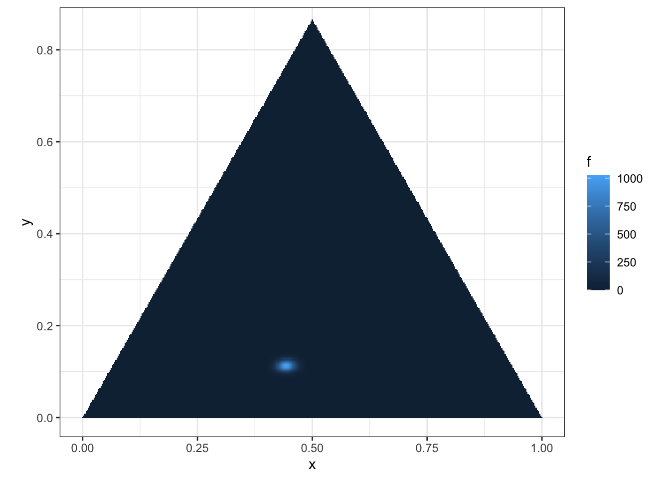
tam <- 26
pac <- pbc <- pcc <- seq(0,1,length=tam)

# Criando o vetor 'rr' que copia length(pbc) vezes cada ponto de 'pac'
rr <- vector()
j <- 1
for(i in 1:tam^2)
{
  if(i>1 & i %% tam == 1) {j <- j + 1}
  rr[i] <- pac[j]
}

# Criando a matriz 'ptc' que combina todos as ternas (rr, pbc, 1-rr-pbc)
ptc <- cbind(rr, pbc, 1-rr-pbc)

# Criando a matriz 'nptc', que conterá apenas as ternas de 'ptc' cuja soma é igual a 1
j <- 0
nptc <- matrix(0 , nrow=dim(ptc)[1], ncol=dim(ptc)[2])
for(i in 1:dim(ptc)[1])
{
  if(ptc[i,3]>0)
  {
    j <- j + 1
    nptc[j,1] <- ptc[i,1]
    nptc[j,2] <- ptc[i,2]
    nptc[j,3] <- ptc[i,3]
  }
}

# Contando quantos pares de 'nptc' são 'NA'
cont <- 0
for(i in 1:dim(nptc)[1])
{
  if(is.na(nptc[i,1]) == TRUE) {cont <- cont+1}
}

# Atribuindo 'nptc' a 'simplex' apenas com os valores não 'NA'
simplex <- nptc[1:(dim(nptc)[1] - cont), ]
colnames(simplex) <- c('theta1', 'theta2', 'theta3')
rgl::plot3d(simplex, col = 'red')

draws <- extraDistr::rdirichlet(2000, alpha = c(493,379,131))
rgl::plot3d(draws, xlim = c(0,1), ylim = c(0,1), zlim = c(0,1), add = TRUE)
# Opção 5
library(desempateTecnico)
if(type_book == 'bookdown::gitbook'){
  rgl::clear3d()
}
n <- c(492,378,130)
simplex3d(pa=n[1]/sum(n), pb=n[2]/sum(n), pc=n[3]/sum(n), n=sum(n), alpha = 0.05)
7.1.1 Onde pode ser usado
Latent Dirichlet Allocation (LDA).
(Blei et al. 2003)
https://www.tidytextmining.com/topicmodeling.html
https://bookdown.org/Maxine/tidy-text-mining/latent-dirichlet-allocation.html
https://towardsdatascience.com/beginners-guide-to-lda-topic-modelling-with-r-e57a5a8e7a25
Chap. 27 ‘Probabilistic grammars and hierarchical Dirichlet processes’, OHagan & West (2010) - The Oxford handbook of applied bayesian analysis pg. 776