10.8 Análise Discriminante

Análise discriminante ou discriminação tem suas origens nos trabalhos de Ronald Fisher (R. A. Fisher 1936), (R. A. Fisher 1938), (R. A. Fisher 1940), e refere-se a um conjunto técnicas multivariadas com o objetivo de separar grupos de observações. É baseada em métodos multivariados, considerando um conjunto de equações de predição baseadas em variáveis independentes. Há dois enfoques típicos em uma análise discriminante:

Classificação, com o intuito de encontrar uma equação preditiva para atribuir novos indivíduos a grupos pré estabelecidos
Discriminação, que tem por objetivo interpretar uma equação preditiva para entender melhor as relações entre as variáveis

A análise discriminante é similar a uma Regressão Linear Múltipla, sendo a que a principal diferença entre estas duas técnicas é que a análise de regressão lida com uma variável dependente contínua, enquanto a análise discriminante deve ter uma variável dependente categórica ou discreta.

10.8.1 Análise Discriminante Linear (LDA)

A LDA assume que os preditores possuem distribuição gaussiana e que as diferentes classes têm médias específicas de classe e mesma (matriz de) variância e covariâncias.

Exemplo 10.22 Classificando espécies de lírio via LDA.

Avaliando a suposição de normalidade por grupo através do teste de Shapiro-Wilk.

by(iris[,1], iris[,5], shapiro.test)

## iris[, 5]: setosa
## 
##  Shapiro-Wilk normality test
## 
## data:  dd[x, ]
## W = 0.9777, p-value = 0.4595
## 
## ----------------------------------------------------------------------------------- 
## iris[, 5]: versicolor
## 
##  Shapiro-Wilk normality test
## 
## data:  dd[x, ]
## W = 0.97784, p-value = 0.4647
## 
## ----------------------------------------------------------------------------------- 
## iris[, 5]: virginica
## 
##  Shapiro-Wilk normality test
## 
## data:  dd[x, ]
## W = 0.97118, p-value = 0.2583

by(iris[,2], iris[,5], shapiro.test)

## iris[, 5]: setosa
## 
##  Shapiro-Wilk normality test
## 
## data:  dd[x, ]
## W = 0.97172, p-value = 0.2715
## 
## ----------------------------------------------------------------------------------- 
## iris[, 5]: versicolor
## 
##  Shapiro-Wilk normality test
## 
## data:  dd[x, ]
## W = 0.97413, p-value = 0.338
## 
## ----------------------------------------------------------------------------------- 
## iris[, 5]: virginica
## 
##  Shapiro-Wilk normality test
## 
## data:  dd[x, ]
## W = 0.96739, p-value = 0.1809

by(iris[,3], iris[,5], shapiro.test)

## iris[, 5]: setosa
## 
##  Shapiro-Wilk normality test
## 
## data:  dd[x, ]
## W = 0.95498, p-value = 0.05481
## 
## ----------------------------------------------------------------------------------- 
## iris[, 5]: versicolor
## 
##  Shapiro-Wilk normality test
## 
## data:  dd[x, ]
## W = 0.966, p-value = 0.1585
## 
## ----------------------------------------------------------------------------------- 
## iris[, 5]: virginica
## 
##  Shapiro-Wilk normality test
## 
## data:  dd[x, ]
## W = 0.96219, p-value = 0.1098

by(iris[,4], iris[,5], shapiro.test)

## iris[, 5]: setosa
## 
##  Shapiro-Wilk normality test
## 
## data:  dd[x, ]
## W = 0.79976, p-value = 8.659e-07
## 
## ----------------------------------------------------------------------------------- 
## iris[, 5]: versicolor
## 
##  Shapiro-Wilk normality test
## 
## data:  dd[x, ]
## W = 0.94763, p-value = 0.02728
## 
## ----------------------------------------------------------------------------------- 
## iris[, 5]: virginica
## 
##  Shapiro-Wilk normality test
## 
## data:  dd[x, ]
## W = 0.95977, p-value = 0.08695

Avaliando a suposição da igualdade da matriz de variâncias e covariâncias através do teste M de Box (Box 1949), (Box 1950). A hipótese sendo testada é \(H_0: \boldsymbol{\Sigma}_1=\boldsymbol{\Sigma}_2=\cdots=\boldsymbol{\Sigma}_k\).

by(iris[,-5], iris[,5], cov)

## iris[, 5]: setosa
##              Sepal.Length Sepal.Width Petal.Length Petal.Width
## Sepal.Length   0.12424898 0.099216327  0.016355102 0.010330612
## Sepal.Width    0.09921633 0.143689796  0.011697959 0.009297959
## Petal.Length   0.01635510 0.011697959  0.030159184 0.006069388
## Petal.Width    0.01033061 0.009297959  0.006069388 0.011106122
## ----------------------------------------------------------------------------------- 
## iris[, 5]: versicolor
##              Sepal.Length Sepal.Width Petal.Length Petal.Width
## Sepal.Length   0.26643265  0.08518367   0.18289796  0.05577959
## Sepal.Width    0.08518367  0.09846939   0.08265306  0.04120408
## Petal.Length   0.18289796  0.08265306   0.22081633  0.07310204
## Petal.Width    0.05577959  0.04120408   0.07310204  0.03910612
## ----------------------------------------------------------------------------------- 
## iris[, 5]: virginica
##              Sepal.Length Sepal.Width Petal.Length Petal.Width
## Sepal.Length   0.40434286  0.09376327   0.30328980  0.04909388
## Sepal.Width    0.09376327  0.10400408   0.07137959  0.04762857
## Petal.Length   0.30328980  0.07137959   0.30458776  0.04882449
## Petal.Width    0.04909388  0.04762857   0.04882449  0.07543265

by(iris[,-5], iris[,5], cor)

## iris[, 5]: setosa
##              Sepal.Length Sepal.Width Petal.Length Petal.Width
## Sepal.Length    1.0000000   0.7425467    0.2671758   0.2780984
## Sepal.Width     0.7425467   1.0000000    0.1777000   0.2327520
## Petal.Length    0.2671758   0.1777000    1.0000000   0.3316300
## Petal.Width     0.2780984   0.2327520    0.3316300   1.0000000
## ----------------------------------------------------------------------------------- 
## iris[, 5]: versicolor
##              Sepal.Length Sepal.Width Petal.Length Petal.Width
## Sepal.Length    1.0000000   0.5259107    0.7540490   0.5464611
## Sepal.Width     0.5259107   1.0000000    0.5605221   0.6639987
## Petal.Length    0.7540490   0.5605221    1.0000000   0.7866681
## Petal.Width     0.5464611   0.6639987    0.7866681   1.0000000
## ----------------------------------------------------------------------------------- 
## iris[, 5]: virginica
##              Sepal.Length Sepal.Width Petal.Length Petal.Width
## Sepal.Length    1.0000000   0.4572278    0.8642247   0.2811077
## Sepal.Width     0.4572278   1.0000000    0.4010446   0.5377280
## Petal.Length    0.8642247   0.4010446    1.0000000   0.3221082
## Petal.Width     0.2811077   0.5377280    0.3221082   1.0000000

library(biotools)
boxM(iris[,-5], iris[,5])

## 
##  Box's M-test for Homogeneity of Covariance Matrices
## 
## data:  iris[, -5]
## Chi-Sq (approx.) = 140.94, df = 20, p-value < 2.2e-16

A diferença significativa (p-value < 2.2e-16) sugere que é mais interessante considerar a QDA, que não faz a suposição de igualdade de matrizes de variâncias e covariâncias. De toda forma procederemos com a LDA para comparação. Inicialmente é obtida a amostra de treino. O número máximo de funções discriminantes úteis que podem separar os \(G\) grupos é o mínimo entre \(G-1\) e \(p\), logo \(\text{min}(3-1,4)=2\).

# amostra de treino: 60%
set.seed(1); itrain <- sort(sample(1:nrow(iris), floor(.6*nrow(iris))))
train <- iris[itrain,]
test <- iris[-itrain,]
table(train$Species)

## 
##     setosa versicolor  virginica 
##         32         26         32

O ajuste do modelo de análise discriminante linear pode ser feito pela função MASS::lda.

library(MASS)
# modelo
fit <- lda(Species ~ ., iris, prior = c(1,1,1)/3, subset = itrain)
fit

## Call:
## lda(Species ~ ., data = iris, prior = c(1, 1, 1)/3, subset = itrain)
## 
## Prior probabilities of groups:
##     setosa versicolor  virginica 
##  0.3333333  0.3333333  0.3333333 
## 
## Group means:
##            Sepal.Length Sepal.Width Petal.Length Petal.Width
## setosa         5.006250    3.428125     1.456250    0.250000
## versicolor     6.007692    2.784615     4.376923    1.334615
## virginica      6.740625    2.968750     5.621875    2.015625
## 
## Coefficients of linear discriminants:
##                    LD1        LD2
## Sepal.Length  0.907457 -0.4936054
## Sepal.Width   1.197211 -1.7603466
## Petal.Length -2.187455  1.2776671
## Petal.Width  -2.815162 -3.1631095
## 
## Proportion of trace:
##    LD1    LD2 
## 0.9907 0.0093

plot(fit)

A predição pode ser realizada através da função genérica stats::predict.

pred <- predict(fit, test)

Pode-se fazer um gráfico bivariado para melhorar a apresentação.

library(ggord)
# dados de treino
ggord(fit, train$Species, ylim = c(-5, 5))

Pode-se criar gráficos por discriminante linear para avaliar a discriminação gerada.

ldahist(data = pred$x[,1], g = test$Species)

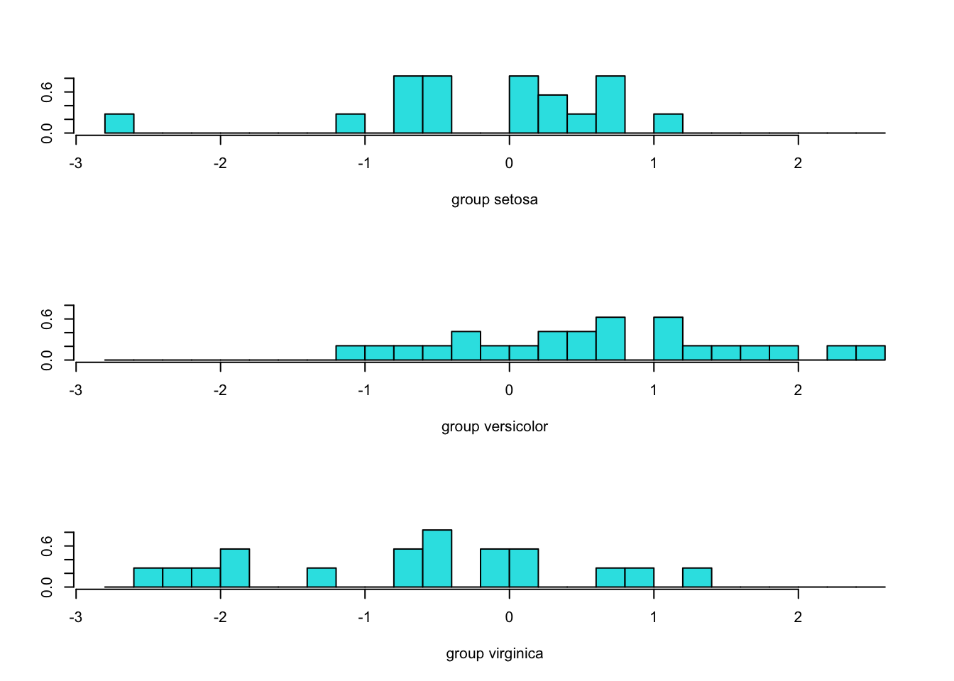
Note que a separação da primeira discriminante linear é muito mais acurada do que a segunda.

ldahist(data = pred$x[,2], g = test$Species)

Pode-se calcular a acurácia da predição do modelo. Pode-se calcular a proporção de atribuições corretas total e por categoria.

# matriz de confusão
(cm <- table(test[,5], pred$class))

##             
##              setosa versicolor virginica
##   setosa         18          0         0
##   versicolor      0         23         1
##   virginica       0          0        18

# relatório via caret::confusionMatrix
caret::confusionMatrix(cm)

## Confusion Matrix and Statistics
## 
##             
##              setosa versicolor virginica
##   setosa         18          0         0
##   versicolor      0         23         1
##   virginica       0          0        18
## 
## Overall Statistics
##                                           
##                Accuracy : 0.9833          
##                  95% CI : (0.9106, 0.9996)
##     No Information Rate : 0.3833          
##     P-Value [Acc > NIR] : < 2.2e-16       
##                                           
##                   Kappa : 0.9748          
##                                           
##  Mcnemar's Test P-Value : NA              
## 
## Statistics by Class:
## 
##                      Class: setosa Class: versicolor Class: virginica
## Sensitivity                    1.0            1.0000           0.9474
## Specificity                    1.0            0.9730           1.0000
## Pos Pred Value                 1.0            0.9583           1.0000
## Neg Pred Value                 1.0            1.0000           0.9762
## Prevalence                     0.3            0.3833           0.3167
## Detection Rate                 0.3            0.3833           0.3000
## Detection Prevalence           0.3            0.4000           0.3000
## Balanced Accuracy              1.0            0.9865           0.9737

Exercício 10.8 Ajuste os modelos LDA, QDA, MDA e FDA no banco de dados wine descrito a seguir.

data(wine, package = 'rattle')

10.8.1.1 Análise Discriminante Linear com penalidades

O pacote TULIP integra métodos populares baseados em LDA de alta dimensão e fornece ferramentas para classificação linear, semiparamétrica e tensor-variável. As funções estão incluídas para ajuste de modelo, validação cruzada e previsão. Motivados por conjuntos de dados com diversas fontes de preditores estão incluídas funções para ajuste de covariáveis.

10.8.2 Análise Discriminante Quadrática (QDA)

O ajuste do modelo de análise discriminante quadrática pode ser feito pela função MASS::qda.

Exemplo 10.23 Classificando espécies de lírio via QDA.

library(MASS)
# modelo
fit <- qda(Species ~ ., iris, prior = c(1,1,1)/3, subset = itrain)
fit

## Call:
## qda(Species ~ ., data = iris, prior = c(1, 1, 1)/3, subset = itrain)
## 
## Prior probabilities of groups:
##     setosa versicolor  virginica 
##  0.3333333  0.3333333  0.3333333 
## 
## Group means:
##            Sepal.Length Sepal.Width Petal.Length Petal.Width
## setosa         5.006250    3.428125     1.456250    0.250000
## versicolor     6.007692    2.784615     4.376923    1.334615
## virginica      6.740625    2.968750     5.621875    2.015625

# predição
pred <- predict(fit, test)
# matriz de confusão
(cm <- table(pred$class, test[,5]))

##             
##              setosa versicolor virginica
##   setosa         18          0         0
##   versicolor      0         22         0
##   virginica       0          2        18

# relatório via caret::confusionMatrix
caret::confusionMatrix(cm)

## Confusion Matrix and Statistics
## 
##             
##              setosa versicolor virginica
##   setosa         18          0         0
##   versicolor      0         22         0
##   virginica       0          2        18
## 
## Overall Statistics
##                                           
##                Accuracy : 0.9667          
##                  95% CI : (0.8847, 0.9959)
##     No Information Rate : 0.4             
##     P-Value [Acc > NIR] : < 2.2e-16       
##                                           
##                   Kappa : 0.9497          
##                                           
##  Mcnemar's Test P-Value : NA              
## 
## Statistics by Class:
## 
##                      Class: setosa Class: versicolor Class: virginica
## Sensitivity                    1.0            0.9167           1.0000
## Specificity                    1.0            1.0000           0.9524
## Pos Pred Value                 1.0            1.0000           0.9000
## Neg Pred Value                 1.0            0.9474           1.0000
## Prevalence                     0.3            0.4000           0.3000
## Detection Rate                 0.3            0.3667           0.3000
## Detection Prevalence           0.3            0.3667           0.3333
## Balanced Accuracy              1.0            0.9583           0.9762

Para gráficos da QDA veja o link https://stackoverflow.com/questions/63782598/quadratic-discriminant-analysis-qda-plot-in-r.

10.8.3 Análise Discriminante Mista (MDA)

(Robert Tibshirani. Original R port by Friedrich Leisch, Hornik, and code. 2020) propõem uma classe mista de análise discriminante.

Exemplo 10.24 Classificando espécies de lírio via MDA.

library(mda)
# modelo
fit <- mda(Species ~ ., data = train)
fit

## Call:
## mda(formula = Species ~ ., data = train)
## 
## Dimension: 4 
## 
## Percent Between-Group Variance Explained:
##     v1     v2     v3     v4 
##  95.56  98.61  99.93 100.00 
## 
## Degrees of Freedom (per dimension): 5 
## 
## Training Misclassification Error: 0.02222 ( N = 90 )
## 
## Deviance: 9.871

# predição
pred <- predict(fit, test)
# matriz de confusão
(cm <- table(pred, test[,5]))

##             
## pred         setosa versicolor virginica
##   setosa         18          0         0
##   versicolor      0         23         1
##   virginica       0          1        17

# relatório via caret::confusionMatrix
caret::confusionMatrix(cm)

## Confusion Matrix and Statistics
## 
##             
## pred         setosa versicolor virginica
##   setosa         18          0         0
##   versicolor      0         23         1
##   virginica       0          1        17
## 
## Overall Statistics
##                                           
##                Accuracy : 0.9667          
##                  95% CI : (0.8847, 0.9959)
##     No Information Rate : 0.4             
##     P-Value [Acc > NIR] : < 2.2e-16       
##                                           
##                   Kappa : 0.9495          
##                                           
##  Mcnemar's Test P-Value : NA              
## 
## Statistics by Class:
## 
##                      Class: setosa Class: versicolor Class: virginica
## Sensitivity                    1.0            0.9583           0.9444
## Specificity                    1.0            0.9722           0.9762
## Pos Pred Value                 1.0            0.9583           0.9444
## Neg Pred Value                 1.0            0.9722           0.9762
## Prevalence                     0.3            0.4000           0.3000
## Detection Rate                 0.3            0.3833           0.2833
## Detection Prevalence           0.3            0.4000           0.3000
## Balanced Accuracy              1.0            0.9653           0.9603

10.8.4 Análise Discriminante Flexível (FDA)

(Robert Tibshirani. Original R port by Friedrich Leisch, Hornik, and code. 2020) propõem uma classe flexível de análise discriminante.

Exemplo 10.25 Classificando espécies de lírio via FDA.

library(mda)
# modelo
fit <- fda(Species ~ ., data = train)
fit

## Call:
## fda(formula = Species ~ ., data = train)
## 
## Dimension: 2 
## 
## Percent Between-Group Variance Explained:
##     v1     v2 
##  99.18 100.00 
## 
## Degrees of Freedom (per dimension): 5 
## 
## Training Misclassification Error: 0.02222 ( N = 90 )

# predição
pred <- predict(fit, test)
# matriz de confusão
(cm <- table(pred, test[,5]))

##             
## pred         setosa versicolor virginica
##   setosa         18          0         0
##   versicolor      0         23         0
##   virginica       0          1        18

# relatório via caret::confusionMatrix
caret::confusionMatrix(cm)

## Confusion Matrix and Statistics
## 
##             
## pred         setosa versicolor virginica
##   setosa         18          0         0
##   versicolor      0         23         0
##   virginica       0          1        18
## 
## Overall Statistics
##                                           
##                Accuracy : 0.9833          
##                  95% CI : (0.9106, 0.9996)
##     No Information Rate : 0.4             
##     P-Value [Acc > NIR] : < 2.2e-16       
##                                           
##                   Kappa : 0.9748          
##                                           
##  Mcnemar's Test P-Value : NA              
## 
## Statistics by Class:
## 
##                      Class: setosa Class: versicolor Class: virginica
## Sensitivity                    1.0            0.9583           1.0000
## Specificity                    1.0            1.0000           0.9762
## Pos Pred Value                 1.0            1.0000           0.9474
## Neg Pred Value                 1.0            0.9730           1.0000
## Prevalence                     0.3            0.4000           0.3000
## Detection Rate                 0.3            0.3833           0.3000
## Detection Prevalence           0.3            0.3833           0.3167
## Balanced Accuracy              1.0            0.9792           0.9881

Referências

Box, George EP. 1949. “A General Distribution Theory for a Class of Likelihood Criteria.” Biometrika 36 (3/4): 317–46. https://www.jstor.org/stable/pdf/2332671.pdf.

———. 1950. “Problems in the Analysis of Growth and Wear Curves.” Biometrics 6 (4): 362–89.

———. 1936. “The Use of Multiple Measurements in Taxonomic Problems.” Annals of Eugenics 7 (2): 179–88. http://rcs.chemometrics.ru/Tutorials/classification/Fisher.pdf.

———. 1938. “The Statistical Utilization of Multiple Measurements.” Annals of Eugenics 8 (4): 376–86. https://digital.library.adelaide.edu.au/dspace/bitstream/2440/15232/1/155.pdf.

———. 1940. “The Precision of Discriminant Functions.” Annals of Eugenics 10 (1): 422–29. https://hekyll.services.adelaide.edu.au/dspace/bitstream/2440/15240/1/175.pdf.

Robert Tibshirani. Original R port by Friedrich Leisch, Trevor Hastie &, Kurt Hornik, and Brian D. Ripley. Balasubramanian Narasimhan has contributed to the upgrading of the code. 2020. Mda: Mixture and Flexible Discriminant Analysis. https://CRAN.R-project.org/package=mda.