9.6 Regressão Linear
A classe de Modelos Lineares atende a uma ampla gama de problemas aplicados, apresentada por (Neter et al. 2005), podendo incluir modelos lineares de séries temporais (Enders 2014). Há generalizações tais como os Modelos Lineares Generalizados (MLG/GLM) (McCullagh and Nelder 1989), Modelos Aditivos Generalizados (MAG/GAM) (Hastie and Tibshirani 1986), dentre outras. (Friedman and Stuetzle 1981) sugerem a Regressão com Perseguição da Projeção, procedimento que modela a superfície de regressão como uma soma de funções de suavização de combinações lineares das variáveis preditoras de forma iterativa. (O’Hagan and Forster 1994, 244–76) e (Paulino et al. 2003, 194–208) fornecem uma abordagem bayesiana para a regressão.
Quando trabalha-se com dados multivariados (i.e., quase sempre), recomenda-se a exploração criteoriosa dos dados. Não raro ocorrem valores faltantes (missings), rotulados por NA na linguagem R conforme Seção NA no Estatística Básica do mesmo autor. Tais valores faltantes podem dificultar os procedimentos de modelagem, e sua ocorrência se soma a outras questões como a multicolinearidade, discutida na Seção 9.6.3.
9.6.1 Clássico
9.6.1.1 Modelo
O modelo de Regressão Linear Múltipla (RLM/MLR) populacional/universal é construído, na abordagem clássica, com todos as \(N\)-uplas da população ou universo, i.e., \((x_{1i},x_{2i},\ldots,x_{pi},y_i), \; i \in \{1,\ldots,N\}\). Pode ser descrito pela Eq. (9.24).
\[\begin{equation} y_i = \beta_0 + \beta_1 x_{1i} + \cdots + \beta_p x_{pi} + \varepsilon_i, \tag{9.24} \end{equation}\] onde \(\varepsilon_i \sim \mathcal{N}(0,\sigma_{\varepsilon})\).
Por ter dimensionalidade \(p\) usualmente utiliza-se notação matricial na forma
\[\begin{equation} Y = X \boldsymbol{\beta} + \boldsymbol{\varepsilon}, \tag{9.25} \end{equation}\]
onde \(Y = \begin{bmatrix} Y_1 \\ Y_2 \\ \vdots \\ Y_n \end{bmatrix}\), \(X = \begin{bmatrix} 1 & x_{11} & x_{12} & \cdots & x_{1p} \\ 1 & x_{21} & x_{22} & \cdots & x_{2p} \\ \vdots & \vdots & \vdots & \ddots & \vdots \\ 1 & x_{n1} & x_{n2} & \cdots & x_{np} \end{bmatrix}\), \(\boldsymbol{\beta} = \begin{bmatrix} \beta_0 \\ \beta_1 \\ \vdots \\ \beta_p \end{bmatrix}\) e \(\boldsymbol{\varepsilon} = \begin{bmatrix} \varepsilon_1 \\ \varepsilon_2 \\ \vdots \\ \varepsilon_n \end{bmatrix}\).
Estimativa dos parâmetros
Para a obtenção das estimativas dos parâmetros utiliza-se a Eq. (9.26). Para ajustar um modelo RPO, basta eliminar a coluna unitária de \(X\). \[\begin{equation} \boldsymbol{\hat{\beta}} = (X'X)^{-1} X'Y \tag{9.26} \end{equation}\]
Exemplo 9.8 Em http://archive.ics.uci.edu/ml/datasets/Energy+efficiency está disponível uma análise de energia feita por (Tsanas and Xifara 2012) usando 12 formas diferentes de construção simuladas no Ecotect. Os edifícios diferem em relação à área envidraçada, à distribuição da área envidraçada e à orientação, entre outros parâmetros. Foram simuladas várias configurações como funções das características acima mencionadas para obter 768 formas de construção. O conjunto de dados detalhado a seguir compreende 768 amostras e 8 características (X1 a X8), com o objetivo de prever duas respostas reais (Y1 e Y2).
X1: Compactação Relativa
X2: Superfície
X3: Área da parede
X4: Área do telhado
X5: Altura total
X6: Orientação
X7: Área de Envidraçamento
X8: Distribuição da Área de Envidraçamento
Y1: Carga de aquecimento
Y2: Carga de resfriamento
# arquivo
url1 = 'http://archive.ics.uci.edu/ml/machine-learning-databases/00242/ENB2012_data.xlsx'
download.file(url1, 'temp.xlsx', mode = 'wb')
energy = readxl::read_excel('temp.xlsx')

# exploratória
skimr::skim(energy)| Name | energy |
| Number of rows | 768 |
| Number of columns | 10 |
| _______________________ | |
| Column type frequency: | |
| numeric | 10 |
| ________________________ | |
| Group variables | None |
Variable type: numeric
| skim_variable | n_missing | complete_rate | mean | sd | p0 | p25 | p50 | p75 | p100 | hist |
|---|---|---|---|---|---|---|---|---|---|---|
| X1 | 0 | 1 | 0.76 | 0.11 | 0.62 | 0.68 | 0.75 | 0.83 | 0.98 | ▇▆▃▃▂ |
| X2 | 0 | 1 | 671.71 | 88.09 | 514.50 | 606.38 | 673.75 | 741.12 | 808.50 | ▅▅▇▅▇ |
| X3 | 0 | 1 | 318.50 | 43.63 | 245.00 | 294.00 | 318.50 | 343.00 | 416.50 | ▃▅▇▂▂ |
| X4 | 0 | 1 | 176.60 | 45.17 | 110.25 | 140.88 | 183.75 | 220.50 | 220.50 | ▃▃▁▁▇ |
| X5 | 0 | 1 | 5.25 | 1.75 | 3.50 | 3.50 | 5.25 | 7.00 | 7.00 | ▇▁▁▁▇ |
| X6 | 0 | 1 | 3.50 | 1.12 | 2.00 | 2.75 | 3.50 | 4.25 | 5.00 | ▇▇▁▇▇ |
| X7 | 0 | 1 | 0.23 | 0.13 | 0.00 | 0.10 | 0.25 | 0.40 | 0.40 | ▂▇▁▇▇ |
| X8 | 0 | 1 | 2.81 | 1.55 | 0.00 | 1.75 | 3.00 | 4.00 | 5.00 | ▇▆▆▆▆ |
| Y1 | 0 | 1 | 22.31 | 10.09 | 6.01 | 12.99 | 18.95 | 31.67 | 43.10 | ▇▇▃▆▅ |
| Y2 | 0 | 1 | 24.59 | 9.51 | 10.90 | 15.62 | 22.08 | 33.13 | 48.03 | ▇▂▅▃▁ |


##
##  Shapiro-Wilk normality test
##
## data:  energy$Y1
## W = 0.9121, p-value < 2.2e-16##
## Call:
## lm(formula = Y1 ~ . - Y2, data = energy)
##
## Residuals:
## Min 1Q Median 3Q Max
## -9.8965 -1.3196 -0.0252 1.3532 7.7052
##
## Coefficients: (1 not defined because of singularities)
## Estimate Std. Error t value Pr(>|t|)
## (Intercept) 84.013418 19.033613 4.414 1.16e-05 ***
## X1 -64.773432 10.289448 -6.295 5.19e-10 ***
## X2 -0.087289 0.017075 -5.112 4.04e-07 ***
## X3 0.060813 0.006648 9.148 < 2e-16 ***
## X4 NA NA NA NA
## X5 4.169954 0.337990 12.338 < 2e-16 ***
## X6 -0.023330 0.094705 -0.246 0.80548
## X7 19.932736 0.813986 24.488 < 2e-16 ***
## X8 0.203777 0.069918 2.915 0.00367 **
## ---
## Signif. codes: 0 '***' 0.001 '**' 0.01 '*' 0.05 '.' 0.1 ' ' 1
##
## Residual standard error: 2.934 on 760 degrees of freedom
## Multiple R-squared: 0.9162, Adjusted R-squared: 0.9154
## F-statistic: 1187 on 7 and 760 DF, p-value: < 2.2e-16No modelo atribuído a fit0, é possível notar que não é possível calcular o coeficiente da variável X4 devido a singularidades. Para mais detalhes, veja esta discussão do Stackoverflow.
Stepwise
O método de regressão stepwise foi proposto por (Efroymson 1960) com o intuito de selecionar variáveis em regressões múltiplas conforme Eq. (9.24). De acordo com o autor10, no procedimento de stepwise os resultados intermediários dos métodos para a obtenção das estimativas de regressões múltiplas “são usados para fornecer informações estatísticas valiosas em cada etapa do cálculo”. O autor também ressalta11 que o método “é baseado nos fatos que (a) uma variável pode ser indicada como significativa em qualquer estágio inicial e, assim, entrar na equação e (b) após várias outras variáveis serem adicionadas à equação de regressão, o variável inicial pode ser indicada como insignificante. A variável insignificante será removida da equação de regressão antes de adicionar uma nova variável. Portanto, apenas variáveis significativas são incluídas na regressão final”.
Este método busca automaticamente o melhor conjunto de variáveis de maneira a minimizar alguma medida. Na implementação de R documentada em stats::step(), o modelo selecionado será aquele com o menor valor de AIC (Akaike 1974) (k = 2) ou BIC (Schwarz 1978) (k = log(n)). Note que ‘seleção de modelos’ e ‘seleção de variáveis’ são sinônimos.
Exemplo 9.9 A partir do modelo saturado do Exemplo 9.8 pode-se ajustar uma regressão stepwise.
##
## Call:
## lm(formula = Y1 ~ X1 + X2 + X3 + X5 + X7 + X8, data = energy)
##
## Residuals:
##     Min      1Q  Median      3Q     Max
## -9.9315 -1.3189 -0.0262  1.3587  7.7169
##
## Coefficients:
##               Estimate Std. Error t value Pr(>|t|)
## (Intercept)  83.931762  19.018978   4.413 1.17e-05 ***
## X1          -64.773432  10.283096  -6.299 5.06e-10 ***
## X2           -0.087289   0.017065  -5.115 3.97e-07 ***
## X3            0.060813   0.006644   9.153  < 2e-16 ***
## X5            4.169954   0.337781  12.345  < 2e-16 ***
## X7           19.932736   0.813484  24.503  < 2e-16 ***
## X8            0.203777   0.069875   2.916  0.00365 **
## ---
## Signif. codes:  0 '***' 0.001 '**' 0.01 '*' 0.05 '.' 0.1 ' ' 1
##
## Residual standard error: 2.933 on 761 degrees of freedom
## Multiple R-squared:  0.9162, Adjusted R-squared:  0.9155
## F-statistic:  1387 on 6 and 761 DF,  p-value: < 2.2e-16
Pelos resultados obtidos pode-se verificar que o modelo ajustado em fit1 possui todas as variávies significativas para um \(\alpha\) inferior a 0.01, estatística F de 1387 para 6 e 761 graus de liberdade, levando a um p-value geral do modelo menor que \(2.2 \times 10^{-16}\), o que indica boa aderência aos dados. O valor do Multiple R-squared é o coeficiente de determinação de valor 0.9162, indicando que o modelo explica em torno de 92% da variação de Y1.
Com este diagnóstico pode-se considerar um modelo aceitável, que possui coeficientes de X1 e X2 negativos, indicando que um aumento destas variáveis (respectivamente compactação relativa e superfície) deve reduzir a carga de aquecimento. Mais especificamente, um aumento de uma unidade na compactação relativa (X1) gera uma redução esperada de 64.77 unidades na carga de aquecimento, mantidas constantes as demais variáveis. As variáveis X3, X5, X7 e X8 possuem coeficientes positivos, levando a um impacto esperado positivo em Y1. Como exemplo, para cada aumento de uma unidade na altura total (X5) espera-se um aumento aproximando de 4.17 unidades na carga de aquecimento. As outras variáveis possuem interpretação análoga, devendo-se sempre observar o sinal dos coeficientes.
9.6.1.2 LASSO
O modelo LASSO (Least Absolute Shrinkage and Selection Operator) também é definido pela Eq. (9.24), porém com coeficientes obtidos ao \[\begin{equation} \text{minimizar} \sum_{i=1}^n (Y_i - \beta_0 - \beta_1 X_{i1} - \beta_2 X_{i2} - \cdots - \beta_p X_{ip})^{2} \\ \text{ sujeito a} \sum_{j=1}^p |\beta_j| \le t \tag{4} \end{equation}\] onde \(t\) é o parâmetro livre ou de regularização.
9.6.1.3 Diagnóstico inferencial
Teste para \(\boldsymbol{\beta}\)
Exemplo 9.10 Considere os dados do Exemplo 9.9. Pode-se gerar um relatório do modelo desejado com base::summary(). Um diagnóstico visual pode ser obtido via base::plot(), onde which=1:4 indica que estão sendo solicitados os 4 primeiros gráficos disponíves de um total de 6.
##
## Call:
## lm(formula = Y1 ~ X1 + X2 + X3 + X5 + X7 + X8, data = energy)
##
## Residuals:
##     Min      1Q  Median      3Q     Max
## -9.9315 -1.3189 -0.0262  1.3587  7.7169
##
## Coefficients:
##               Estimate Std. Error t value Pr(>|t|)
## (Intercept)  83.931762  19.018978   4.413 1.17e-05 ***
## X1          -64.773432  10.283096  -6.299 5.06e-10 ***
## X2           -0.087289   0.017065  -5.115 3.97e-07 ***
## X3            0.060813   0.006644   9.153  < 2e-16 ***
## X5            4.169954   0.337781  12.345  < 2e-16 ***
## X7           19.932736   0.813484  24.503  < 2e-16 ***
## X8            0.203777   0.069875   2.916  0.00365 **
## ---
## Signif. codes:  0 '***' 0.001 '**' 0.01 '*' 0.05 '.' 0.1 ' ' 1
##
## Residual standard error: 2.933 on 761 degrees of freedom
## Multiple R-squared:  0.9162, Adjusted R-squared:  0.9155
## F-statistic:  1387 on 6 and 761 DF,  p-value: < 2.2e-16
9.6.1.4 Diagnóstico preditivo
Exemplo 9.11 Considere novamente os dados do Exemplo ??.
# arquivo
url1 = 'http://archive.ics.uci.edu/ml/machine-learning-databases/00242/ENB2012_data.xlsx'
download.file(url1, 'temp.xlsx', mode = 'wb')
energy = readxl::read_excel('temp.xlsx')

# treino-teste
set.seed(999)
itrain <- sort(sample(1:nrow(energy), ceiling(0.7*nrow(energy))))
train <- energy[itrain,]
test <- energy[-itrain,]

# modelo
fit0 <- lm(Y1 ~ . -Y2, data = train)
fit1 <- step(fit0, trace = 0)

# predição
pred <- predict(fit1, test)

# resíduos de predição
r <- pred-test$Y1 # predito - realizado
(mse <- mean(r^2)) # https://en.wikipedia.org/wiki/Mean_squared_error
## [1] 9.330395## [1] 3.05457## [1] 2.219659## [1] 0.1052415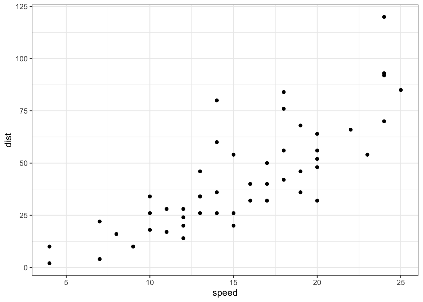
# 100 repetições
M <- 100
residuos <- data.frame(modelo=1:M, mse=NA, rmse=NA, mae=NA, mape=NA)
for(i in 1:M){
  # treino-teste
  set.seed(i)
  itrain <- sort(sample(1:nrow(energy), ceiling(0.7*nrow(energy))))
  train <- energy[itrain,]
  test <- energy[-itrain,]

  # modelo
  fit0 <- lm(Y1 ~ . -Y2, data = train)
  fit1 <- step(fit0, trace=0)

  # predição
  pred <- predict(fit1, test)

  # resíduos de predição
  r <- pred-test$Y1
  residuos[i,2] <- mean(r^2)
  residuos[i,3] <- sqrt(residuos[i,2])
  residuos[i,4] <- mean(abs(r))
  residuos[i,5] <- mean(abs(r/test$Y1))
}
par(mfrow=c(2,2))
hist(residuos[,2], main = 'MSE', 30)
hist(residuos[,3], main = 'RMSE', 30)
hist(residuos[,4], main = 'MAE', 30)
hist(residuos[,5], main = 'MAPE', 30)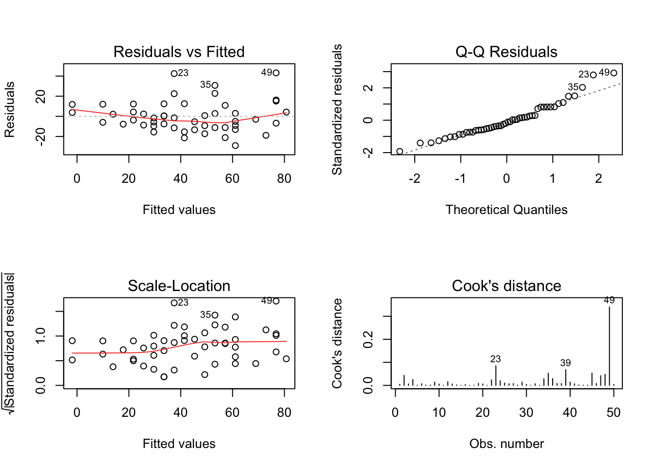
| Name | residuos |
| Number of rows | 100 |
| Number of columns | 5 |
| _______________________ | |
| Column type frequency: | |
| numeric | 5 |
| ________________________ | |
| Group variables | None |
Variable type: numeric
| skim_variable | n_missing | complete_rate | mean | sd | p0 | p25 | p50 | p75 | p100 | hist |
|---|---|---|---|---|---|---|---|---|---|---|
| modelo | 0 | 1 | 50.50 | 29.01 | 1.00 | 25.75 | 50.50 | 75.25 | 100.00 | ▇▇▇▇▇ |
| mse | 0 | 1 | 8.65 | 0.85 | 6.55 | 8.12 | 8.61 | 9.22 | 11.37 | ▂▇▇▃▁ |
| rmse | 0 | 1 | 2.94 | 0.14 | 2.56 | 2.85 | 2.93 | 3.04 | 3.37 | ▂▅▇▅▁ |
| mae | 0 | 1 | 2.08 | 0.10 | 1.84 | 2.02 | 2.07 | 2.15 | 2.42 | ▂▇▆▃▁ |
| mape | 0 | 1 | 0.10 | 0.01 | 0.09 | 0.09 | 0.10 | 0.10 | 0.12 | ▃▇▅▁▁ |
Exercício 9.2 Veja as seguintes documentações.
chemCal::inverse.predict(Ranke 2022)
Exercício 9.3 Acesse o endereço http://archive.ics.uci.edu/ml/datasets.php e escolha um banco de dados com mais de 100 atributos (variáveis/colunas). Faça análises considerando modelos lineares e, se pertinente, utilizando componentes principais. \(\\\)
Exercício 9.4 Refaça o Exemplo 9.8 utilizando a variável Y2 como resposta, ajustando o modelo saturado, filtrando as variáveis com a função step e interpretando os resultados.
Exemplo 9.12 (Belsley et al. 2004, 39) analisam a hipótese desenvolvida por (Modigliani and Papademos 1975), de que a a razão de poupança ao longo da vida (poupança pessoal agregada dividido pelo rendimento disponível) é explicada pelo rendimento disponível per capita, a taxa de variação percentual do rendimento disponível per capita e duas variáveis demográficas: a proporção da população com menos de 15 anos e a proporção da população com mais de 75 anos. Os dados são calculados ao longo da década de 1960-1970 para remover o ciclo de negócios ou outras flutuações de curto prazo.

hist(LifeCycleSavings$sr, 30)
qqnorm(LifeCycleSavings$sr)
qqline(LifeCycleSavings$sr, col = 'red')
shapiro.test(LifeCycleSavings$sr)
##
## Shapiro-Wilk normality test
##
## data: LifeCycleSavings$sr
## W = 0.98074, p-value = 0.5836##
## Call:
## lm(formula = sr ~ pop15 + pop75 + ddpi, data = LifeCycleSavings)
##
## Residuals:
## Min 1Q Median 3Q Max
## -8.2539 -2.6159 -0.3913 2.3344 9.7070
##
## Coefficients:
## Estimate Std. Error t value Pr(>|t|)
## (Intercept) 28.1247 7.1838 3.915 0.000297 ***
## pop15 -0.4518 0.1409 -3.206 0.002452 **
## pop75 -1.8354 0.9984 -1.838 0.072473 .
## ddpi 0.4278 0.1879 2.277 0.027478 *
## ---
## Signif. codes: 0 '***' 0.001 '**' 0.01 '*' 0.05 '.' 0.1 ' ' 1
##
## Residual standard error: 3.767 on 46 degrees of freedom
## Multiple R-squared: 0.3365, Adjusted R-squared: 0.2933
## F-statistic: 7.778 on 3 and 46 DF, p-value: 0.0002646##
## Call:
## omcdiag(mod = mod, Inter = TRUE, detr = detr, red = red, conf = conf,
## theil = theil, cn = cn)
##
##
## Overall Multicollinearity Diagnostics
##
## MC Results detection
## Determinant |X'X|: 0.1739 0
## Farrar Chi-Square: 82.4971 1
## Red Indicator: 0.5254 1
## Sum of Lambda Inverse: 12.4857 0
## Theil's Method: 0.9827 1
## Condition Number: 31.7169 1
##
## 1 --> COLLINEARITY is detected by the test
## 0 --> COLLINEARITY is not detected by the test## pop15 pop75 ddpi
## 5.745478 5.736014 1.004186
Exercício 9.5 Considere o Exemplo 9.12.
a. A partir da saída de car::vif, você recomenda retirar alguma variável do modelo? Em caso afirmativo, execute sua recomendação.
b. Teste jtools::summ(fm1).
Exemplo 9.13 Considere o banco de dados disponível em https://archive.ics.uci.edu/dataset/162/forest+fires baseado em (Cortez and Morais 2007).
X- x-axis spatial coordinate within the Montesinho park map: 1 to 9Y- y-axis spatial coordinate within the Montesinho park map: 2 to 9month- month of the year: ‘jan’ to ‘dec’day- day of the week: ‘mon’ to ‘sun’FFMC- FFMC index from the FWI system: 18.7 to 96.20DMC- DMC index from the FWI system: 1.1 to 291.3DC- DC index from the FWI system: 7.9 to 860.6ISI- ISI index from the FWI system: 0.0 to 56.10temp- temperature in Celsius degrees: 2.2 to 33.30RH- relative humidity in %: 15.0 to 100wind- wind speed in km/h: 0.40 to 9.40rain- outside rain in mm/m2 : 0.0 to 6.4area- the burned area of the forest (in ha): 0.00 to 1090.84 (this output variable is very skewed towards 0.0, thus it may make sense to model with the logarithm transform).
dat <- read.table('https://filipezabala.com/data/forestfires.csv',
                 sep = ',', head = TRUE)
head(dat)
## X Y month day FFMC DMC DC ISI temp RH wind rain area
## 1 7 5 mar fri 86.2 26.2 94.3 5.1 8.2 51 6.7 0.0 0
## 2 7 4 oct tue 90.6 35.4 669.1 6.7 18.0 33 0.9 0.0 0
## 3 7 4 oct sat 90.6 43.7 686.9 6.7 14.6 33 1.3 0.0 0
## 4 8 6 mar fri 91.7 33.3 77.5 9.0 8.3 97 4.0 0.2 0
## 5 8 6 mar sun 89.3 51.3 102.2 9.6 11.4 99 1.8 0.0 0
## 6 8 6 aug sun 92.3 85.3 488.0 14.7 22.2 29 5.4 0.0 0##
## 1 2 3 4 5 6 7 8 9
## 48 73 55 91 30 86 60 61 13## 'data.frame': 517 obs. of 13 variables:
## $ X : Ord.factor w/ 9 levels "1"<"2"<"3"<"4"<..: 7 7 7 8 8 8 8 8 8 7 ...
## $ Y : Ord.factor w/ 7 levels "2"<"3"<"4"<"5"<..: 4 3 3 5 5 5 5 5 5 4 ...
## $ month: chr "mar" "oct" "oct" "mar" ...
## $ day : chr "fri" "tue" "sat" "fri" ...
## $ FFMC : num 86.2 90.6 90.6 91.7 89.3 92.3 92.3 91.5 91 92.5 ...
## $ DMC : num 26.2 35.4 43.7 33.3 51.3 ...
## $ DC : num 94.3 669.1 686.9 77.5 102.2 ...
## $ ISI : num 5.1 6.7 6.7 9 9.6 14.7 8.5 10.7 7 7.1 ...
## $ temp : num 8.2 18 14.6 8.3 11.4 22.2 24.1 8 13.1 22.8 ...
## $ RH : int 51 33 33 97 99 29 27 86 63 40 ...
## $ wind : num 6.7 0.9 1.3 4 1.8 5.4 3.1 2.2 5.4 4 ...
## $ rain : num 0 0 0 0.2 0 0 0 0 0 0 ...
## $ area : num 0 0 0 0 0 0 0 0 0 0 ...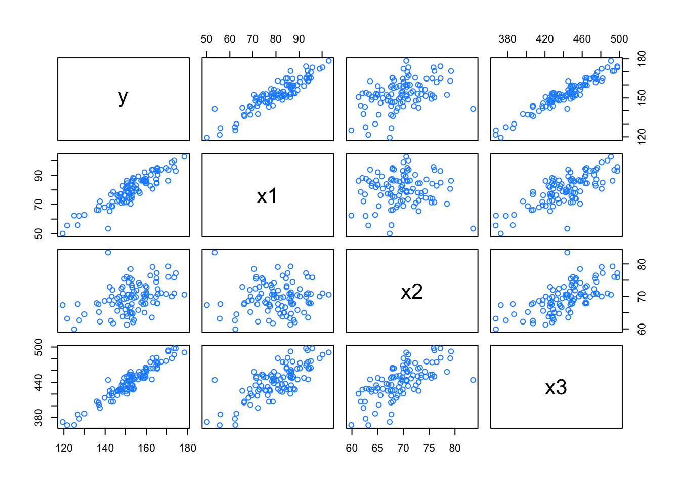
##
## Call:
## lm(formula = area ~ temp, data = dat)
##
## Residuals:
##     Min      1Q  Median      3Q     Max
##  -27.34  -14.68  -10.39   -3.42 1071.33
##
## Coefficients:
##             Estimate Std. Error t value Pr(>|t|)
## (Intercept)  -7.4138     9.4996  -0.780   0.4355
## temp          1.0726     0.4808   2.231   0.0261 *
## ---
## Signif. codes:  0 '***' 0.001 '**' 0.01 '*' 0.05 '.' 0.1 ' ' 1
##
## Residual standard error: 63.41 on 515 degrees of freedom
## Multiple R-squared:  0.009573,   Adjusted R-squared:  0.00765
## F-statistic: 4.978 on 1 and 515 DF,  p-value: 0.0261
# modelando log area
fit2 <- lm(larea ~ ., data = dat[,-13]) # tirando a coluna 13, area
fit3 <- step(fit2, trace = 0)
summary(fit3)
##
## Call:
## lm(formula = larea ~ X + Y + month + DMC + DC + temp + wind,
## data = dat[, -13])
##
## Residuals:
## Min 1Q Median 3Q Max
## -2.1879 -0.9764 -0.4079 0.7768 5.3173
##
## Coefficients:
## Estimate Std. Error t value Pr(>|t|)
## (Intercept) 0.780632 0.575046 1.358 0.175247
## X.L 0.984402 0.345491 2.849 0.004567 **
## X.Q 1.229688 0.339002 3.627 0.000317 ***
## X.C 0.453981 0.291630 1.557 0.120191
## X^4 0.406301 0.259677 1.565 0.118317
## X^5 0.377971 0.224246 1.686 0.092529 .
## X^6 -0.116953 0.219999 -0.532 0.595241
## X^7 0.233594 0.174057 1.342 0.180203
## X^8 -0.564175 0.218151 -2.586 0.009994 **
## Y.L 0.188704 0.713436 0.264 0.791507
## Y.Q -1.551066 0.453561 -3.420 0.000679 ***
## Y.C -2.270578 0.674401 -3.367 0.000821 ***
## Y^4 -2.771889 0.808894 -3.427 0.000663 ***
## Y^5 -1.888967 0.609695 -3.098 0.002059 **
## Y^6 -0.753255 0.304775 -2.472 0.013795 *
## monthaug 0.643724 0.788255 0.817 0.414531
## monthdec 2.213019 0.773107 2.863 0.004384 **
## monthfeb 0.365346 0.551503 0.662 0.507993
## monthjan -0.682928 1.076240 -0.635 0.526020
## monthjul 0.436781 0.683625 0.639 0.523176
## monthjun -0.394812 0.630963 -0.626 0.531786
## monthmar -0.230436 0.493123 -0.467 0.640495
## monthmay 0.736262 1.056583 0.697 0.486240
## monthnov -0.967716 1.428329 -0.678 0.498400
## monthoct 1.315924 0.957744 1.374 0.170079
## monthsep 1.360462 0.887515 1.533 0.125952
## DMC 0.004546 0.001774 2.563 0.010675 *
## DC -0.002498 0.001231 -2.029 0.042954 *
## temp 0.023922 0.014498 1.650 0.099583 .
## wind 0.058852 0.036372 1.618 0.106294
## ---
## Signif. codes: 0 '***' 0.001 '**' 0.01 '*' 0.05 '.' 0.1 ' ' 1
##
## Residual standard error: 1.345 on 487 degrees of freedom
## Multiple R-squared: 0.1268, Adjusted R-squared: 0.07477
## F-statistic: 2.438 on 29 and 487 DF, p-value: 6e-05# retirar coordenadas X e Y
fit4 <- lm(larea ~ ., data = dat[,-c(1:3,13)]) # tirando a colunas 1,2, 13
fit5 <- step(fit4, trace = 0)
summary(fit5)##
## Call:
## lm(formula = larea ~ DMC + RH + wind, data = dat[, -c(1:3, 13)])
##
## Residuals:
## Min 1Q Median 3Q Max
## -1.5093 -1.1071 -0.6537 0.9216 5.7712
##
## Coefficients:
## Estimate Std. Error t value Pr(>|t|)
## (Intercept) 0.9129363 0.2433065 3.752 0.000195 ***
## DMC 0.0017552 0.0009657 1.817 0.069731 .
## RH -0.0055830 0.0037785 -1.478 0.140138
## wind 0.0624134 0.0345109 1.809 0.071112 .
## ---
## Signif. codes: 0 '***' 0.001 '**' 0.01 '*' 0.05 '.' 0.1 ' ' 1
##
## Residual standard error: 1.392 on 513 degrees of freedom
## Multiple R-squared: 0.01425, Adjusted R-squared: 0.008485
## F-statistic: 2.472 on 3 and 513 DF, p-value: 0.061019.6.2 Bayesiano
Uma prévia pode ser encontrada https://alpopkes.com/posts/machine_learning/bayesian_linear_regression/
Exemplo 9.14 Ajustando os modelos lineares clássico e bayesiano para o banco de dados datasets::cars.

##
## Call:
## lm(formula = dist ~ speed, data = cars)
##
## Residuals:
##     Min      1Q  Median      3Q     Max
## -29.069  -9.525  -2.272   9.215  43.201
##
## Coefficients:
##             Estimate Std. Error t value Pr(>|t|)
## (Intercept) -17.5791     6.7584  -2.601   0.0123 *
## speed         3.9324     0.4155   9.464 1.49e-12 ***
## ---
## Signif. codes:  0 '***' 0.001 '**' 0.01 '*' 0.05 '.' 0.1 ' ' 1
##
## Residual standard error: 15.38 on 48 degrees of freedom
## Multiple R-squared:  0.6511, Adjusted R-squared:  0.6438
## F-statistic: 89.57 on 1 and 48 DF,  p-value: 1.49e-12
# Regressão linear bayesiana via `rstanarm::stan_glm`
library(rstan)
library(rstanarm)
options(mc.cores = parallel::detectCores())

fit_stan <- rstanarm::stan_glm(dist ~ speed, data = cars, family = gaussian)
rstan::stan_trace(fit_stan, pars = c('(Intercept)', 'speed', 'sigma'))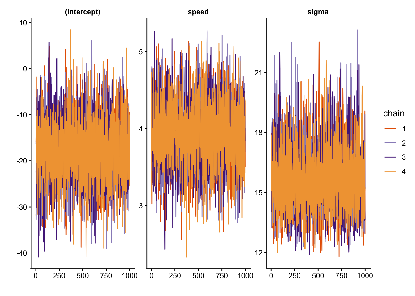
##
## Model Info:
##  function:     stan_glm
##  family:       gaussian [identity]
##  formula:      dist ~ speed
##  algorithm:    sampling
##  sample:       4000 (posterior sample size)
##  priors:       see help('prior_summary')
##  observations: 50
##  predictors:   2
##
## Estimates:
##               mean   sd    10%   50%   90%
## (Intercept) -17.6    7.0 -26.5 -17.6  -8.8
## speed         3.9    0.4   3.4   3.9   4.5
## sigma        15.7    1.6  13.7  15.5  17.8
##
## Fit Diagnostics:
##            mean   sd   10%   50%   90%
## mean_PPD 42.9    3.1 39.0  43.0  46.7
##
## The mean_ppd is the sample average posterior predictive distribution of the outcome variable (for details see help('summary.stanreg')).
##
## MCMC diagnostics
##               mcse Rhat n_eff
## (Intercept)   0.1  1.0  3711
## speed         0.0  1.0  3651
## sigma         0.0  1.0  3483
## mean_PPD      0.0  1.0  4213
## log-posterior 0.0  1.0  1591
##
## For each parameter, mcse is Monte Carlo standard error, n_eff is a crude measure of effective sample size, and Rhat is the potential scale reduction factor on split chains (at convergence Rhat=1).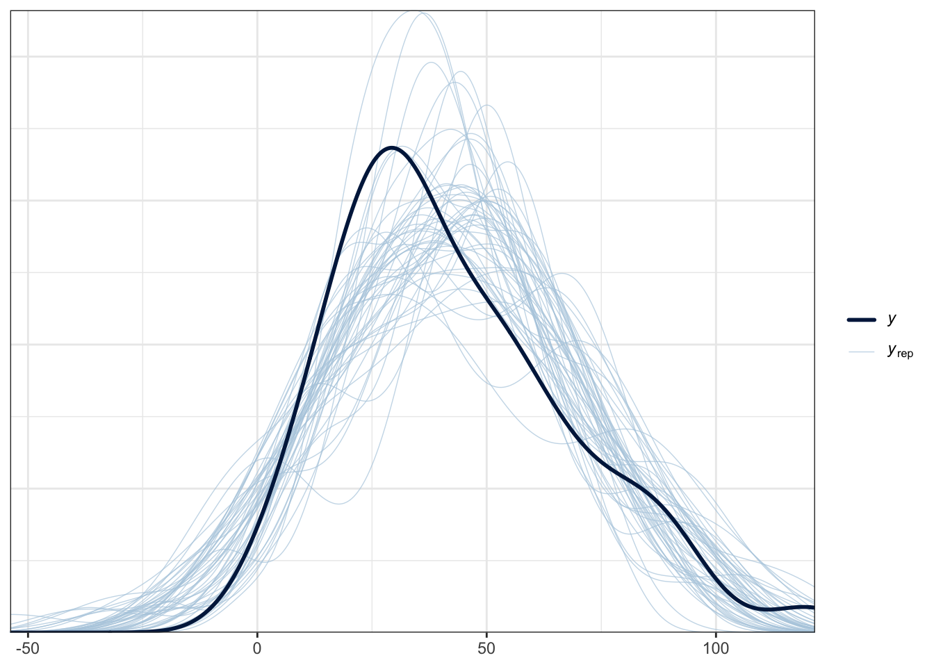
rstanarm::posterior_vs_prior(fit_stan, group_by_parameter = TRUE,
                             pars = c('(Intercept)', 'speed', 'sigma'))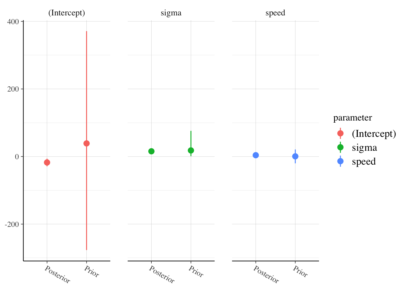
Exercício 9.6 Veja as seguintes documentações:
a. ?rstanarm::print.stanreg.
b. ?rstanarm::prior_summary.
c. ?rstanarm::summary.stanreg.
d. ?rstanarm::pp_check.
e. ?rstanarm::launch_shinystan.
f. ?rstanarm::posterior_vs_prior.
9.6.3 Multicolinearidade
Segundo (Everitt and Skrondal 2006), multicolinearidade é um termo utilizado na análise de regressão para indicar situações em que as variáveis explicativas estão relacionadas por uma função linear, impossibilitando a estimação dos coeficientes de regressão.
Exemplo 9.15 Dalpiaz (2022) - Applied Statistics with R traz alguns exemplos sobre colinearidade.
gen_exact_collin_data <- function(num_samples = 100) {
  x1 = rnorm(n = num_samples, mean = 80, sd = 10)
  x2 = rnorm(n = num_samples, mean = 70, sd = 5)
  x3 = 2 * x1 + 4 * x2 + 3
  y = 3 + x1 + x2 + rnorm(n = num_samples, mean = 0, sd = 1)
  data.frame(y, x1, x2, x3)
}

set.seed(42)
col_data <- gen_exact_collin_data()
head(col_data)
## y x1 x2 x3
## 1 170.7135 93.70958 76.00483 494.4385
## 2 152.9106 74.35302 75.22376 452.6011
## 3 152.7866 83.63128 64.98396 430.1984
## 4 170.6306 86.32863 79.24241 492.6269
## 5 152.3320 84.04268 66.66613 437.7499
## 6 151.3155 78.93875 70.52757 442.9878
##            y         x1         x2        x3
## y  1.0000000 0.91124848 0.43068603 0.9557550
## x1 0.9112485 1.00000000 0.03127984 0.7638609
## x2 0.4306860 0.03127984 1.00000000 0.6689586
## x3 0.9557550 0.76386089 0.66895856 1.0000000## y x1 x2 x3
## y 1
## x1 * 1
## x2 . 1
## x3 B , , 1
## attr(,"legend")
## [1] 0 ' ' 0.3 '.' 0.6 ',' 0.8 '+' 0.9 '*' 0.95 'B' 1##
## Call:
## lm(formula = y ~ x1 + x2 + x3, data = col_data)
##
## Residuals:
## Min 1Q Median 3Q Max
## -2.57662 -0.66188 -0.08253 0.63706 2.52057
##
## Coefficients: (1 not defined because of singularities)
## Estimate Std. Error t value Pr(>|t|)
## (Intercept) 2.957336 1.735165 1.704 0.0915 .
## x1 0.985629 0.009788 100.702 <2e-16 ***
## x2 1.017059 0.022545 45.112 <2e-16 ***
## x3 NA NA NA NA
## ---
## Signif. codes: 0 '***' 0.001 '**' 0.01 '*' 0.05 '.' 0.1 ' ' 1
##
## Residual standard error: 1.014 on 97 degrees of freedom
## Multiple R-squared: 0.9923, Adjusted R-squared: 0.9921
## F-statistic: 6236 on 2 and 97 DF, p-value: < 2.2e-16X <- cbind(1, as.matrix(col_data[,-1]))
fit1 <- lm(y ~ x1 + x2, data = col_data)
fit2 <- lm(y ~ x1 + x3, data = col_data)
fit3 <- lm(y ~ x2 + x3, data = col_data)
all.equal(fitted(fit1), fitted(fit2))## [1] TRUE## [1] TRUE9.6.3.1 Pacote mctest
O pacote mctest (Imdad et al. 2019) pode ser utilizado para calcular medidas de diagnóstico de multicolinearidade populares e amplamente utilizadas.
Exemplo 9.16 (Woods et al. 1932) estudam a associação do calor evoluído durante a fabricação de 13 misturas de cimento de quatro ingredientes básicos. Cada porcentagem de ingrediente parece ser arredondada para um número inteiro. A soma das quatro porcentagens de mistura varia 95% a 99%. Se todas as quatro variáveis \(X\) do regressor sempre somassem 100%, a matriz \(X\) centrada seria então de posto 3. A primeira coluna é a resposta e as quatro colunas restantes são os preditores.
Y: Calor (cals/gm) evoluído na composição.
X1: Porcentagem inteira de \(3Ca O Al_2 O_3\) na mistura.
X2: Porcentagem inteira de \(3Ca O Si O_2\) na mistura.
X3: Porcentagem inteira de \(4Ca O Al_2 O_3 Fe_2 O_3\) na mistura.
X4: Porcentagem inteira de \(2Ca O Si O_2\) na mistura.
library(mctest)
data(Hald) ## Hald Cement data
model <- lm(y ~ ., data = as.data.frame(Hald))
## Medidas de diagnóstico geral e autovalores com intercepto
mctest(model)
##
## Call:
## omcdiag(mod = mod, Inter = TRUE, detr = detr, red = red, conf = conf,
## theil = theil, cn = cn)
##
##
## Overall Multicollinearity Diagnostics
##
## MC Results detection
## Determinant |X'X|: 0.0011 1
## Farrar Chi-Square: 67.2825 1
## Red Indicator: 0.5414 1
## Sum of Lambda Inverse: 622.3006 1
## Theil's Method: 0.9981 1
## Condition Number: 249.5783 1
##
## 1 --> COLLINEARITY is detected by the test
## 0 --> COLLINEARITY is not detected by the test##
## Call:
## imcdiag(mod = mod, method = method, corr = FALSE, vif = vif,
## tol = tol, conf = conf, cvif = cvif, ind1 = ind1, ind2 = ind2,
## leamer = leamer, all = all)
##
##
## All Individual Multicollinearity Diagnostics Result
##
## VIF TOL Wi Fi Leamer CVIF Klein IND1 IND2
## X1 38.4962 0.0260 112.4886 187.4811 0.1612 -0.5846 0 0.0087 0.9875
## X2 254.4232 0.0039 760.2695 1267.1158 0.0627 -3.8635 1 0.0013 1.0099
## X3 46.8684 0.0213 137.6052 229.3419 0.1461 -0.7117 0 0.0071 0.9923
## X4 282.5129 0.0035 844.5386 1407.5643 0.0595 -4.2900 1 0.0012 1.0103
##
## 1 --> COLLINEARITY is detected by the test
## 0 --> COLLINEARITY is not detected by the test
##
## X1 , X2 , X3 , X4 , coefficient(s) are non-significant may be due to multicollinearity
##
## R-square of y on all x: 0.9824
##
## * use method argument to check which regressors may be the reason of collinearity
## ===================================9.6.3.2 Fator de Inflação da Variância (VIF)
(Chatterjee and Hadi 2012, 248–51) definem o Fator de Inflação da Variância (VIF - Variance Inflation Factor) para a variável \(X_j\) tal que
\[\begin{equation} VIF_j = \frac{1}{1-r_{j}^2}, \; j=1,\ldots,p \tag{9.27} \end{equation}\]
onde \(r_{j}^2\) é o coeficiente de determinação que resulta quando a variável preditora \(X_j\) é regredida contra todas as outras variáveis preditoras. Se \(X_j\) tiver um forte relacionamento linear com as outras variáveis preditoras, \(r_{j}^2\) deve ficar próximo de 1 e \(VIF_j\) seria grande. Como regra de bolso, valores de \(VIF\) maiores que 10 geralmente são tomados como um sinal de que os dados têm problema de colinearidade.
9.6.3.4 Diagnóstico de Belsley, Kuh e Welsch
(Belsley et al. 2004, 112–52) sugerem um procedimento de diagnóstico para detectar colinearidade em matrizes \(X\).
References
“In the stepwise procedure, to be described below, intermediate results, which are not even recorded by normal calculation methods, are used to give valuable statistical information at each step in the calculation. These intermediate answers are also used to control the method of calculation.”↩︎
“An important property of the stepwise procedure is based on the facts that (a) a variable may be indicated to be significant in any early stage and thus enter the equation, and (b) after several other variables are added to the regression equation, the initial variable may be indicated to be insignificant. The insignificant variable will be removed from the regression equation before adding an additional variable. Therefore, only significant variables are included in the final regression.”↩︎