11.12 Modelos ARCH

11.12.1 ARCH

(Engle 1982) propõe o modelo ARCH (Autoregressive Conditional Heteroscedasticity), que permite modelar a variância condicional de uma série em função dos quadrados dos retornos passados. A variância inconstante ao longo do tempo é chamada heterocedasticidade.

O modelo ARCH(\(s\)) pode ser expresso por

\[\begin{equation} y_t = a_t \tag{11.35} \end{equation}\]

\[\begin{equation} a_t = \varepsilon_t \sqrt{h_t} \tag{11.36} \end{equation}\]

\[\begin{equation} h_t = \alpha_0 + \sum_{i=1}^s \alpha_i y_{t-i}^2 \tag{11.37} \end{equation}\]

\[\begin{equation} \varepsilon_t \sim WN(0,1) \tag{11.38} \end{equation}\]

Demonstra-se que \(a_t \sim WN(0,\sigma^2_a)\), i.e., \(a_t\) tem variância constante tal que

\[\begin{equation} \sigma^2_a = \frac{\alpha_0}{1-\sum_{i=1}^s \alpha_i} \tag{11.39} \end{equation}\]

Portanto \(a_t\) possui estacionariedade fraca ou de segunda ordem. Para mais detalhes recomenda-se (Engle 1982), (Shephard 1996) e (Box et al. 2008, 413).

11.12.1.1 Clássico

Exemplo 11.54 Adaptado das documentações de tseries::garch() (Trapletti and Hornik 2024) e rugarch::ugarchspec() (Galanos 2025), simulando e ajustando um modelo ARCH\((2)\).

# libs
library(tseries)
library(rugarch)

# número de observações simuladas, 100 primeiras descartadas
n <- 1100

# coeficientes ARCH(2): alfa_0=0.1, alfa_1=0.5 e alfa_2=0.2
a <- c(0.1, 0.5, 0.2)

# \varepsilon_t, Eq. 11.38
set.seed(42); e <- rnorm(n) 

# vetor para conter a série temporal yt simulada (double-precision vector)
y <- double(n)

# \sigma_a^2,  Eq. 11.39
sigma2a <- sqrt(a[1]/(1-a[2]-a[3]))

# 2 primeiros valores de yt, Eq. 11.35
set.seed(314); y[1:2] <- rnorm(2, sd = sigma2a)

# gera processo ARCH(2)
for(i in 3:n){
  # Eq. 11.37
  ht <- a[1] + a[2]*y[i-1]^2 + a[3]*y[i-2]^2
  # Eqs. 11.35 e 11.36
  y[i] <- e[i]*sqrt(ht)
}

# descartando as 100 primeiras observações
y <- ts(y[101:n])

# ARCH(2) 
spec <- ugarchspec(variance.model = list(garchOrder = c(2,0)),
                   mean.model = list(armaOrder = c(0,0)))
fit_arch <- ugarchfit(spec, y)

# diagnóstico
fit_arch

## 
## *---------------------------------*
## *          GARCH Model Fit        *
## *---------------------------------*
## 
## Conditional Variance Dynamics    
## -----------------------------------
## GARCH Model  : sGARCH(2,0)
## Mean Model   : ARFIMA(0,0,0)
## Distribution : norm 
## 
## Optimal Parameters
## ------------------------------------
##         Estimate  Std. Error  t value Pr(>|t|)
## mu     -0.015908    0.012160  -1.3082 0.190817
## omega   0.095962    0.009116  10.5266 0.000000
## alpha1  0.500585    0.063300   7.9082 0.000000
## alpha2  0.225688    0.049399   4.5686 0.000005
## 
## Robust Standard Errors:
##         Estimate  Std. Error  t value Pr(>|t|)
## mu     -0.015908    0.011578  -1.3739 0.169473
## omega   0.095962    0.009047  10.6065 0.000000
## alpha1  0.500585    0.063524   7.8802 0.000000
## alpha2  0.225688    0.057314   3.9378 0.000082
## 
## LogLikelihood : -661.2625 
## 
## Information Criteria
## ------------------------------------
##                    
## Akaike       1.3305
## Bayes        1.3502
## Shibata      1.3305
## Hannan-Quinn 1.3380
## 
## Weighted Ljung-Box Test on Standardized Residuals
## ------------------------------------
##                         statistic p-value
## Lag[1]                    0.06124  0.8045
## Lag[2*(p+q)+(p+q)-1][2]   0.16723  0.8747
## Lag[4*(p+q)+(p+q)-1][5]   1.17259  0.8195
## d.o.f=0
## H0 : No serial correlation
## 
## Weighted Ljung-Box Test on Standardized Squared Residuals
## ------------------------------------
##                         statistic p-value
## Lag[1]                      0.197  0.6571
## Lag[2*(p+q)+(p+q)-1][5]     3.104  0.3884
## Lag[4*(p+q)+(p+q)-1][9]     6.582  0.2367
## d.o.f=2
## 
## Weighted ARCH LM Tests
## ------------------------------------
##             Statistic Shape Scale P-Value
## ARCH Lag[3]    0.1861 0.500 2.000  0.6662
## ARCH Lag[5]    1.9632 1.440 1.667  0.4794
## ARCH Lag[7]    3.8599 2.315 1.543  0.3672
## 
## Nyblom stability test
## ------------------------------------
## Joint Statistic:  0.5701
## Individual Statistics:              
## mu     0.02503
## omega  0.35415
## alpha1 0.25326
## alpha2 0.21252
## 
## Asymptotic Critical Values (10% 5% 1%)
## Joint Statistic:          1.07 1.24 1.6
## Individual Statistic:     0.35 0.47 0.75
## 
## Sign Bias Test
## ------------------------------------
##                    t-value   prob sig
## Sign Bias           1.1810 0.2379    
## Negative Sign Bias  0.9791 0.3278    
## Positive Sign Bias  0.3806 0.7035    
## Joint Effect        1.5812 0.6637    
## 
## 
## Adjusted Pearson Goodness-of-Fit Test:
## ------------------------------------
##   group statistic p-value(g-1)
## 1    20     16.00       0.6573
## 2    30     30.98       0.3664
## 3    40     37.68       0.5300
## 4    50     47.80       0.5218
## 
## 
## Elapsed time : 0.08645487

# previsão 20 períodos à frente
fcast <- ugarchforecast(fit_arch, n.ahead = 20)
plot(fcast, which = 1) # 1 = Conditional mean forecast

11.12.2 GARCH

(Bollerslev 1986) estendeu o trabalho original de Engle, propondo o modelo GARCH (Generalized Autoregressive Conditional Heteroscedasticity), que permite que a variância condicional não dependa somente dos quadrados dos retornos passados, mas também da própria variância passada. O modelo GARCH\((r,s)\) é definido pelas Eq. (11.35), (11.36) e (11.38), com \(h_t\) dado pela Eq. (11.40).

\[\begin{equation} h_t = \alpha_0 + \sum_{i=1}^s \alpha_i y_{t-i}^2 + \sum_{i=1}^r \beta_i h_{t-i} \tag{11.40} \end{equation}\]

Para esta formulação \(a_t\) também possui variância constante, definida pela Eq. (11.41).

\[\begin{equation} \sigma^2_a = \frac{\alpha_0}{1-\sum_{i=1}^s \alpha_i - \sum_{i=1}^r \beta_i} \tag{11.41} \end{equation}\]

11.12.2.1 Clássico

Exemplo 11.55 Adaptado da documentação de tseries::garch(), simulando e ajustando um modelo GARCH(1,1). Lembre-se que “[t]he [a]utocovariances [d]o [n]ot [a]lways [d]ecrease” (Francq and Zakoian 2010, 51).

# libs
library(tseries)
library(rugarch)

# número de observações simuladas, 100 primeiras descartadas
n <- 1100

# coeficientes ARCH(1): alfa_0=0.1 e alfa_1=0.5
a <- c(0.1, 0.5)

# coeficiente GARCH(s,1): beta_1=0.3
b <- c(0.3)

# \varepsilon_t, Eq. 11.38
set.seed(42); e <- rnorm(n)

# vetor para conter a série temporal yt simulada (double-precision vector)
y <- double(n)

# vetor para conter a série temporal de ht
h <- double(n) 

# Eqs. 11.34 e 11.40
set.seed(314); y[1] <- rnorm(1, sd = sqrt(a[1]/(1-a[2]-b[1])))

# gera processo GARCH(1,1)
for(i in 2:n){
  # Eq. 11.39
  h[i] <- a[1] + a[2]*y[i-1]^2 + b[1]*h[i-1] 
  # Eqs. 11.34 e 11.35
  y[i] <- e[i]*sqrt(h[i])
}

# descartando as 100 primeiras observações
y <- ts(y[101:n])

# GARCH(1,1) 
spec <- ugarchspec(variance.model = list(garchOrder = c(1,1)),
                   mean.model = list(armaOrder = c(0,0)))
fit_garch <- ugarchfit(spec, y)

# diagnóstico
fit_garch

## 
## *---------------------------------*
## *          GARCH Model Fit        *
## *---------------------------------*
## 
## Conditional Variance Dynamics    
## -----------------------------------
## GARCH Model  : sGARCH(1,1)
## Mean Model   : ARFIMA(0,0,0)
## Distribution : norm 
## 
## Optimal Parameters
## ------------------------------------
##         Estimate  Std. Error  t value Pr(>|t|)
## mu     -0.018259    0.014908  -1.2248  0.22064
## omega   0.073548    0.014315   5.1377  0.00000
## alpha1  0.468977    0.061610   7.6121  0.00000
## beta1   0.397669    0.061347   6.4823  0.00000
## 
## Robust Standard Errors:
##         Estimate  Std. Error  t value Pr(>|t|)
## mu     -0.018259    0.014069  -1.2978 0.194346
## omega   0.073548    0.017321   4.2462 0.000022
## alpha1  0.468977    0.070549   6.6475 0.000000
## beta1   0.397669    0.084187   4.7236 0.000002
## 
## LogLikelihood : -866.4694 
## 
## Information Criteria
## ------------------------------------
##                    
## Akaike       1.7409
## Bayes        1.7606
## Shibata      1.7409
## Hannan-Quinn 1.7484
## 
## Weighted Ljung-Box Test on Standardized Residuals
## ------------------------------------
##                         statistic p-value
## Lag[1]                    0.05405  0.8162
## Lag[2*(p+q)+(p+q)-1][2]   0.17145  0.8721
## Lag[4*(p+q)+(p+q)-1][5]   1.21927  0.8084
## d.o.f=0
## H0 : No serial correlation
## 
## Weighted Ljung-Box Test on Standardized Squared Residuals
## ------------------------------------
##                         statistic p-value
## Lag[1]                      0.872  0.3504
## Lag[2*(p+q)+(p+q)-1][5]     4.705  0.1783
## Lag[4*(p+q)+(p+q)-1][9]     7.756  0.1437
## d.o.f=2
## 
## Weighted ARCH LM Tests
## ------------------------------------
##             Statistic Shape Scale P-Value
## ARCH Lag[3]  0.000114 0.500 2.000  0.9915
## ARCH Lag[5]  3.394667 1.440 1.667  0.2374
## ARCH Lag[7]  4.871646 2.315 1.543  0.2378
## 
## Nyblom stability test
## ------------------------------------
## Joint Statistic:  0.4709
## Individual Statistics:              
## mu     0.02895
## omega  0.22996
## alpha1 0.30454
## beta1  0.28856
## 
## Asymptotic Critical Values (10% 5% 1%)
## Joint Statistic:          1.07 1.24 1.6
## Individual Statistic:     0.35 0.47 0.75
## 
## Sign Bias Test
## ------------------------------------
##                    t-value   prob sig
## Sign Bias           1.5441 0.1229    
## Negative Sign Bias  1.0226 0.3067    
## Positive Sign Bias  0.7825 0.4341    
## Joint Effect        2.4511 0.4842    
## 
## 
## Adjusted Pearson Goodness-of-Fit Test:
## ------------------------------------
##   group statistic p-value(g-1)
## 1    20     18.20       0.5091
## 2    30     25.88       0.6319
## 3    40     45.84       0.2096
## 4    50     54.80       0.2640
## 
## 
## Elapsed time : 0.04700303

# previsão 20 períodos à frente
fcast <- ugarchforecast(fit_garch, n.ahead = 20)
plot(fcast, which = 1) # 1 = Conditional mean forecast

11.12.2.2 Bayesiano

A função bayesforecast::garch() (Matamoros and Torres 2020) implementa um modelo GARCH\((s,k,h)\) baseado em (Ardia and Hoogerheide 2010) e (Fonseca et al. 2019). As três componentes \((s,k,h) \equiv (s,r,h)\) são a ordem do ARCH (\(s\)), a ordem do GARCH (\(k \equiv r\)) e a ordem do MGARCH (\(h\)) (Bollerslev et al. 1988). Segundo a documentação, as prioris padrão utilizadas no modelo MGARCH são:

• ar ~ normal(0,0.5)
• ma ~ normal(0,0.5)
• mu0 ~ t-student(0,2.5,6)
• sigma0 ~ t-student(0,1,7)
• arch ~ normal(0,0.5)
• garch ~ normal(0,0.5)
• mgarch ~ normal(0,0.5)
• dfv ~ gamma(2,0.1)
• breg ~ t-student(0,2.5,6)

Para mais detalhes veja (Engle Robert and Kevin 2001) e (Engle 2002).

Exemplo 11.56 Considere a série \(y_t\) gerada no Exemplo 11.55.

# libs
library(bayesforecast)

# GARCH(1,1)
fit_garch_bayes <- bayesforecast::garch(y, order = c(1,1,0))
fit_garch_varstan <- bayesforecast::varstan(fit_garch_bayes, iter = 500, 
                                            chains = 1, quiet = TRUE)

## 
## SAMPLING FOR MODEL 'tgarch' NOW (CHAIN 1).
## Chain 1: 
## Chain 1: Gradient evaluation took 0.002354 seconds
## Chain 1: 1000 transitions using 10 leapfrog steps per transition would take 23.54 seconds.
## Chain 1: Adjust your expectations accordingly!
## Chain 1: 
## Chain 1: 
## Chain 1: Iteration:   1 / 500 [  0%]  (Warmup)
## Chain 1: Iteration:  50 / 500 [ 10%]  (Warmup)
## Chain 1: Iteration: 100 / 500 [ 20%]  (Warmup)
## Chain 1: Iteration: 150 / 500 [ 30%]  (Warmup)
## Chain 1: Iteration: 200 / 500 [ 40%]  (Warmup)
## Chain 1: Iteration: 250 / 500 [ 50%]  (Warmup)
## Chain 1: Iteration: 251 / 500 [ 50%]  (Sampling)
## Chain 1: Iteration: 300 / 500 [ 60%]  (Sampling)
## Chain 1: Iteration: 350 / 500 [ 70%]  (Sampling)
## Chain 1: Iteration: 400 / 500 [ 80%]  (Sampling)
## Chain 1: Iteration: 450 / 500 [ 90%]  (Sampling)
## Chain 1: Iteration: 500 / 500 [100%]  (Sampling)
## Chain 1: 
## Chain 1:  Elapsed Time: 0.616 seconds (Warm-up)
## Chain 1:                0.358 seconds (Sampling)
## Chain 1:                0.974 seconds (Total)
## Chain 1:

summary(fit_garch_varstan)

##             mean     se        5%       95%      ess   Rhat
## mu0      -0.0145 0.0009   -0.0383    0.0099 265.6395 0.9996
## sigma0    0.0828 0.0010    0.0583    0.1106 283.0997 0.9983
## arch      0.4844 0.0036    0.4055    0.5701 234.7433 1.0200
## garch     0.3662 0.0036    0.2781    0.4588 181.7439 1.0094
## loglik -869.9343 0.0964 -873.0877 -868.2888 273.2528 0.9986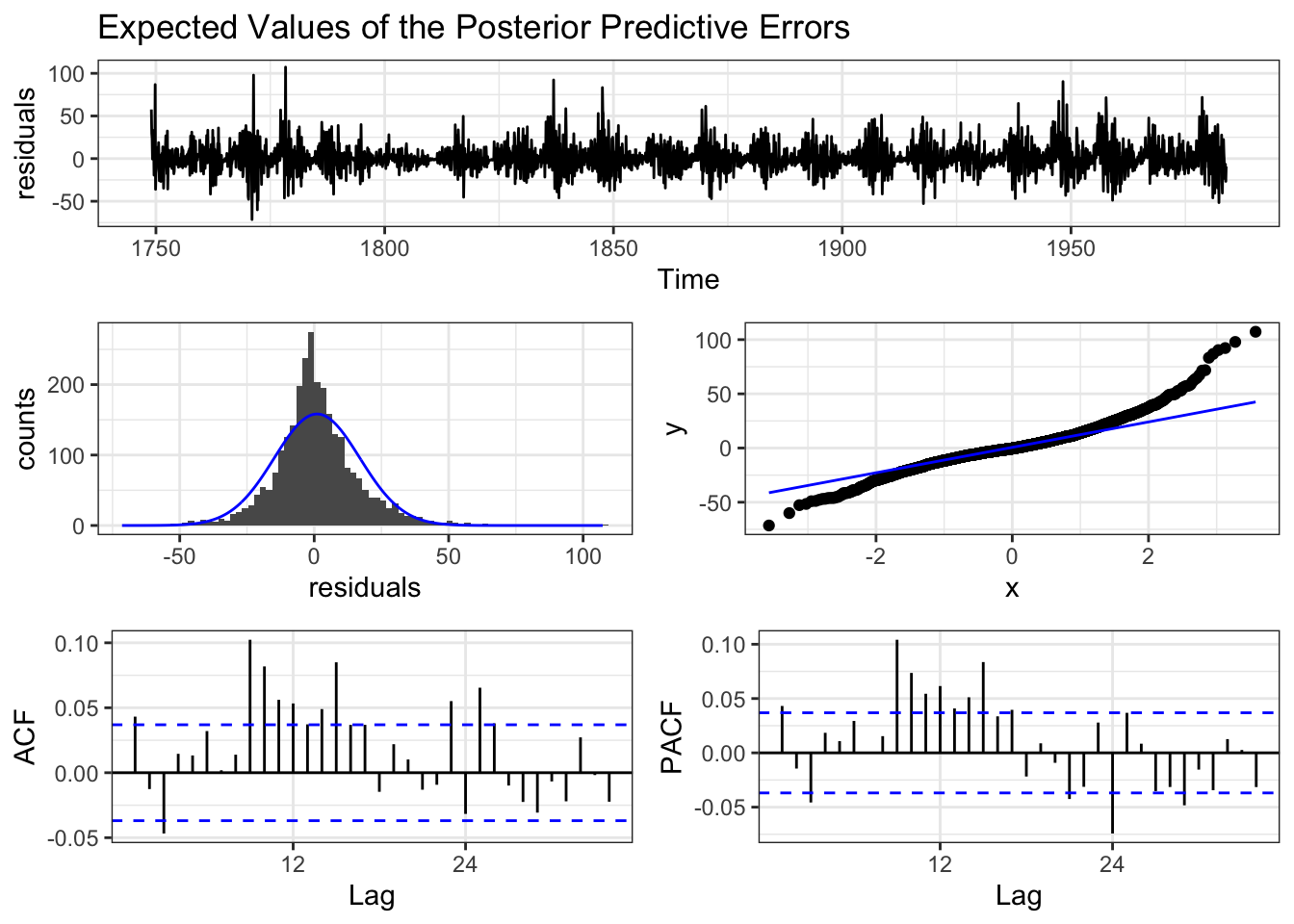

# análise de resíduos
check_residuals(fit_garch_varstan)

# previsão 20 períodos à frente
autoplot(bayesforecast::forecast(fit_garch_varstan, h = 20))

#### Diagnóstico

Ao ajustar um modelo bayesiano usando bayesforecast (que usa internamente Stan), o resumo do objeto ajustado inclui estatísticas de diagnóstico para cada parâmetro estimado. Dois dos principais são ess e Rhat.

---

ess: Effective Sample Size

Definição: O tamanho efetivo da amostra (ESS) mede quanta informação independente suas cadeias MCMC contêm para um parâmetro.

Intuição: Mesmo que você extraia, digamos, 2000 amostras de cada cadeia, as amostras são autocorrelacionadas (não independentes). O ESS informa a quantas amostras independentes suas cadeias são efetivamente equivalentes.

Interpretação: - ESS mais alto → estimativas posterioris mais confiáveis. - Como regra geral: - ESS > 1000 por parâmetro → bom. - ESS < 100 → indica forte autocorrelação; considere executar cadeias mais longas ou melhorar a amostragem.

bayesforecast relata ambos: - ess_bulk: para a parte central (volume) da posteriori. - ess_tail: para as caudas (valores extremos) da posteriori. —

11.12.2.2.1 Rhat: Fator Potencial de Redução de Escala

Definição: Rhat compara a variância entre cadeias com a variância dentro da cadeia para cada parâmetro. É conhecido como estatística de Gelman-Rubin.

Intuição: Se múltiplas cadeias se misturaram bem e convergiram para o mesmo posterior, suas variâncias devem ser semelhantes → Rhat ≈ 1.

Interpretação: - Rhat ≈ 1.00 → boa convergência. - Rhat > 1.00 → possível não convergência, indicam que você deve executar novamente ou reespecificar o modelo. —

Exercício 11.32

1. No Exemplo 11.54 verifique a equivalência entre os modelos ARCH\((2)\), GARCH\((0,2)\) de tseries e GARCH\((2,0,0)\) de bayesforecast.
2. Veja https://asael697.r-universe.dev/bayesforecast.
3. Veja https://cran.r-universe.dev/bayesforecast/doc/manual.html.
4. Veja http://fmwww.bc.edu/EC-C/S2014/823/EC823.S2014.nn09.slides.pdf.

11.12.3 IGARCH

Engle and Bollerslev (1986) propõem o modelo IGARCH, “uma nova classe de modelos definidos para serem integrados em variância” a partir da restrição \(\sum_{i=1}^{s} \alpha_i + \sum_{i=1}^{r} \beta_i = 1\) na Eq. (11.40).

11.12.4 EGARCH

Nelson (1991) propõe o modelo EGARCH com o objetivo de “acomodar a relação assimétrica entre os retornos das ações e as mudanças na volatilidade”. Seguindo a notação de Vrontos et al. (2000),

\[\begin{equation} \log h_t = \alpha_0 + \sum_{i=1}^s \theta_i a_{t-i} + \gamma_i (|a_{t-i}|-E|a_{t-i}|) + \sum_{i=1}^r \beta_i h_{t-i} \tag{11.42} \end{equation}\]

\[\begin{equation} E|a_{t-i}| = \frac{\Gamma(\frac{2}{\nu})}{[\Gamma(\frac{1}{\nu}) \Gamma(\frac{3}{\nu})]^{1/2}} \tag{11.43} \end{equation}\]

11.12.5 ARMA-GARCH

Exemplo 11.57 Considere a série temporal r unlist(tsdl::meta_tsdl[20,2][[1]][[1]]) apresentada por r tsdl::meta_tsdl[20,1], disponível em tsdl::tsdl[[20]]²².

library(forecast)
library(bayesforecast)
# ajustando um modelo ARIMA automático
y <- tsdl::tsdl[[20]]
# ARIMA(2,1,2)
forecast::auto.arima(y)

## Series: y 
## ARIMA(2,1,2) 
## 
## Coefficients:
##          ar1      ar2      ma1     ma2
##       1.3467  -0.3963  -1.7710  0.8103
## s.e.  0.0303   0.0287   0.0205  0.0194
## 
## sigma^2 = 243.8:  log likelihood = -11745.5
## AIC=23500.99   AICc=23501.01   BIC=23530.71

# ajustando ARMA(2,2)-GARCH(1,1) para a série com uma diferença via bayesforecast
fit_garch_bayes <- bayesforecast::garch(y, order = c(1,1,0), arma = c(2,2))
fit_garch_varstan <- bayesforecast::varstan(fit_garch_bayes, iter = 500, chains = 1)

## 
## SAMPLING FOR MODEL 'tgarch' NOW (CHAIN 1).
## Chain 1: Rejecting initial value:
## Chain 1:   Log probability evaluates to log(0), i.e. negative infinity.
## Chain 1:   Stan can't start sampling from this initial value.
## Chain 1: 
## Chain 1: Gradient evaluation took 0.008172 seconds
## Chain 1: 1000 transitions using 10 leapfrog steps per transition would take 81.72 seconds.
## Chain 1: Adjust your expectations accordingly!
## Chain 1: 
## Chain 1: 
## Chain 1: Iteration:   1 / 500 [  0%]  (Warmup)
## Chain 1: Iteration:  50 / 500 [ 10%]  (Warmup)
## Chain 1: Iteration: 100 / 500 [ 20%]  (Warmup)
## Chain 1: Iteration: 150 / 500 [ 30%]  (Warmup)
## Chain 1: Iteration: 200 / 500 [ 40%]  (Warmup)
## Chain 1: Iteration: 250 / 500 [ 50%]  (Warmup)
## Chain 1: Iteration: 251 / 500 [ 50%]  (Sampling)
## Chain 1: Iteration: 300 / 500 [ 60%]  (Sampling)
## Chain 1: Iteration: 350 / 500 [ 70%]  (Sampling)
## Chain 1: Iteration: 400 / 500 [ 80%]  (Sampling)
## Chain 1: Iteration: 450 / 500 [ 90%]  (Sampling)
## Chain 1: Iteration: 500 / 500 [100%]  (Sampling)
## Chain 1: 
## Chain 1:  Elapsed Time: 27.039 seconds (Warm-up)
## Chain 1:                33.128 seconds (Sampling)
## Chain 1:                60.167 seconds (Total)
## Chain 1: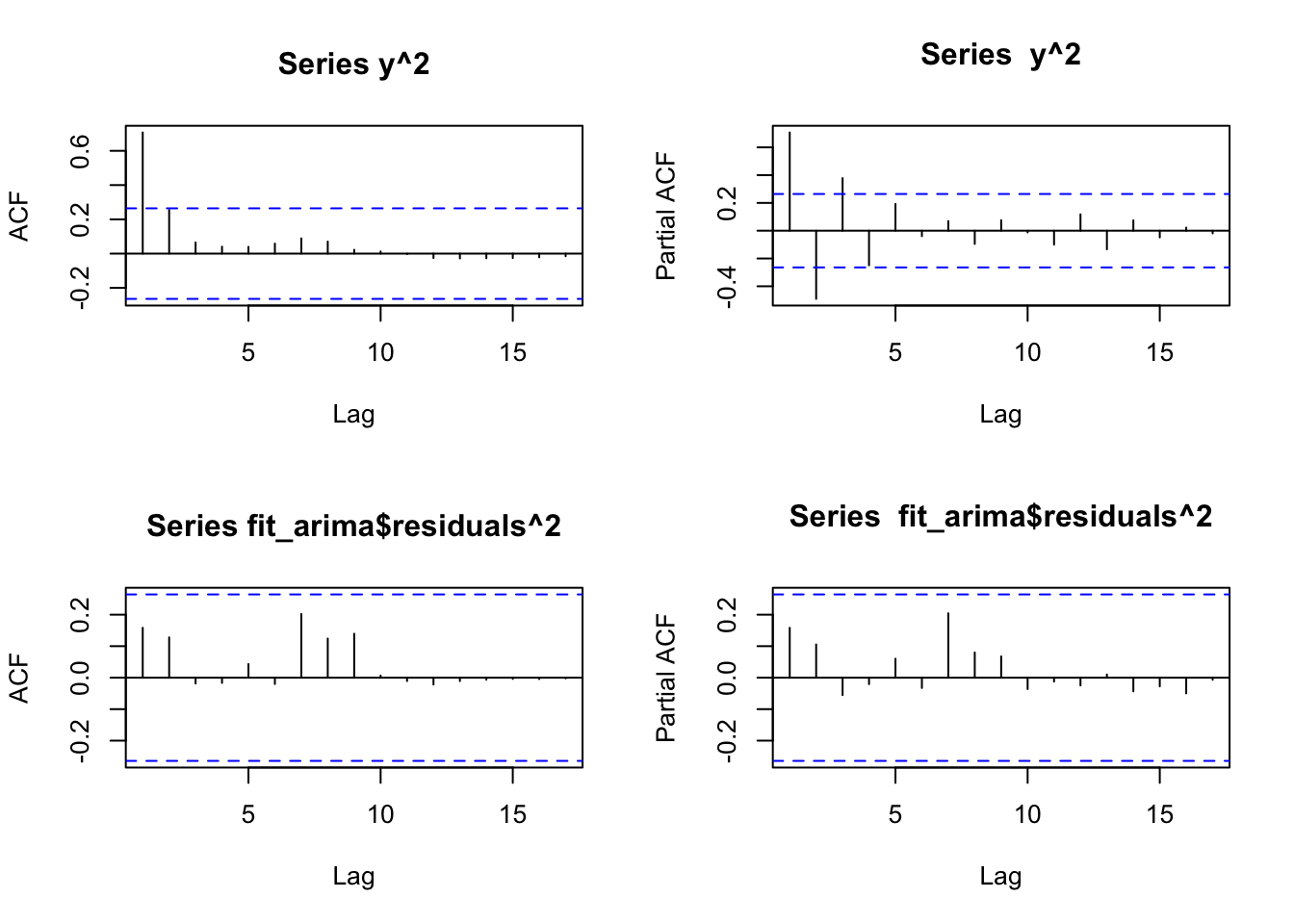

# análise de resíduos
check_residuals(fit_garch_varstan)

# projetando 48 passos
autoplot(bayesforecast::forecast(fit_garch_varstan, h = 48))

# # tomando uma diferença da série
# ydiff <- diff(y)
# fit_garch_bayes_diff <- bayesforecast::garch(ydiff, order = c(1,1,0), arma = c(2,2)) # ajusta ARMA(2,2)-GARCH(1,1)
# fit_garch_varstan_diff <- bayesforecast::varstan(fit_garch_bayes_diff, iter = 500, chains = 1)
# check_residuals(fit_garch_varstan_diff) # análise de resíduos
# bf <- bayesforecast::forecast(fit_garch_varstan_diff, h = 48)
#  # desfazendo as diferenças
# bf$x <- diffinv(bf$x, xi = y[1])
# bf$mean <- diffinv(bf$mean, xi = y[length(y)])
# autoplot(bf) # projetando 48 passos

A função rugarch::ugarchspec() (Galanos 2025) permite ajustar um modelo ARFIMA-GARCH, com variantes do modelo GARCH e variáveis externas (veja documentação).

# libs
library(forecast)
library(rugarch)
# ajustando um modelo ARIMA automático
y <- tsdl::tsdl[[37]]
# ARIMA(1,1,1)
(fit_arima <- forecast::auto.arima(y))

## Series: y 
## ARIMA(1,1,1) 
## 
## Coefficients:
##           ar1     ma1
##       -0.5322  0.9476
## s.e.   0.1389  0.0657
## 
## sigma^2 = 95.43:  log likelihood = -199.28
## AIC=404.57   AICc=405.05   BIC=410.54

# avaliando a série ao quadrado e os resíduos ao quadrado do ARIMA(1,1,1)
par(mfrow=c(2,2))
acf(y^2)
pacf(y^2)
acf(fit_arima$residuals^2)
pacf(fit_arima$residuals^2)

# tomando uma diferença da série
ydiff <- diff(y)
# ajustando ARMA-GARCH para a série com uma diferença via rugarch
spec <- ugarchspec(
  mean.model = list(armaOrder = c(2,2), arfima = FALSE),
  variance.model = list(garchOrder = c(0,1))
)
fit_garch <- ugarchfit(spec = spec, data = y, solver.control = list(trace=0))
fit_garch

## 
## *---------------------------------*
## *          GARCH Model Fit        *
## *---------------------------------*
## 
## Conditional Variance Dynamics    
## -----------------------------------
## GARCH Model  : sGARCH(0,1)
## Mean Model   : ARFIMA(2,0,2)
## Distribution : norm 
## 
## Optimal Parameters
## ------------------------------------
##        Estimate  Std. Error   t value Pr(>|t|)
## mu     9.766928    0.729527  13.38803  0.00000
## ar1    0.973898    0.396542   2.45598  0.01405
## ar2    0.315426    0.525520   0.60022  0.54836
## ma1   -0.033163    0.048437  -0.68466  0.49356
## ma2   -1.091586    0.082845 -13.17617  0.00000
## omega  0.744128    5.858005   0.12703  0.89892
## beta1  0.999000    0.082035  12.17775  0.00000
## 
## Robust Standard Errors:
##        Estimate  Std. Error   t value Pr(>|t|)
## mu     9.766928     1.68982  5.779859 0.000000
## ar1    0.973898     1.37428  0.708662 0.478534
## ar2    0.315426     1.83710  0.171698 0.863675
## ma1   -0.033163     0.15565 -0.213058 0.831282
## ma2   -1.091586     0.29994 -3.639348 0.000273
## omega  0.744128    23.03233  0.032308 0.974226
## beta1  0.999000     0.32684  3.056497 0.002239
## 
## LogLikelihood : -190.7872 
## 
## Information Criteria
## ------------------------------------
##                    
## Akaike       7.1923
## Bayes        7.4477
## Shibata      7.1645
## Hannan-Quinn 7.2911
## 
## Weighted Ljung-Box Test on Standardized Residuals
## ------------------------------------
##                          statistic p-value
## Lag[1]                      0.5043  0.4776
## Lag[2*(p+q)+(p+q)-1][11]    4.4613  0.9972
## Lag[4*(p+q)+(p+q)-1][19]    8.3803  0.7387
## d.o.f=4
## H0 : No serial correlation
## 
## Weighted Ljung-Box Test on Standardized Squared Residuals
## ------------------------------------
##                         statistic p-value
## Lag[1]                      6.099 0.01352
## Lag[2*(p+q)+(p+q)-1][2]     7.204 0.01052
## Lag[4*(p+q)+(p+q)-1][5]     9.123 0.01541
## d.o.f=1
## 
## Weighted ARCH LM Tests
## ------------------------------------
##             Statistic Shape Scale P-Value
## ARCH Lag[2]     2.055 0.500 2.000  0.1517
## ARCH Lag[4]     3.418 1.397 1.611  0.2100
## ARCH Lag[6]     3.772 2.222 1.500  0.3403
## 
## Nyblom stability test
## ------------------------------------
## Joint Statistic:  13.3381
## Individual Statistics:             
## mu    0.03699
## ar1   0.03213
## ar2   0.03140
## ma1   0.03472
## ma2   0.06054
## omega 0.58634
## beta1 0.46952
## 
## Asymptotic Critical Values (10% 5% 1%)
## Joint Statistic:          1.69 1.9 2.35
## Individual Statistic:     0.35 0.47 0.75
## 
## Sign Bias Test
## ------------------------------------
##                     t-value     prob sig
## Sign Bias           0.06203 0.950788    
## Negative Sign Bias  3.02330 0.003938 ***
## Positive Sign Bias  1.64256 0.106749    
## Joint Effect       14.34114 0.002476 ***
## 
## 
## Adjusted Pearson Goodness-of-Fit Test:
## ------------------------------------
##   group statistic p-value(g-1)
## 1    20     17.36       0.5652
## 2    30     25.18       0.6688
## 3    40     30.09       0.8463
## 4    50     44.09       0.6720
## 
## 
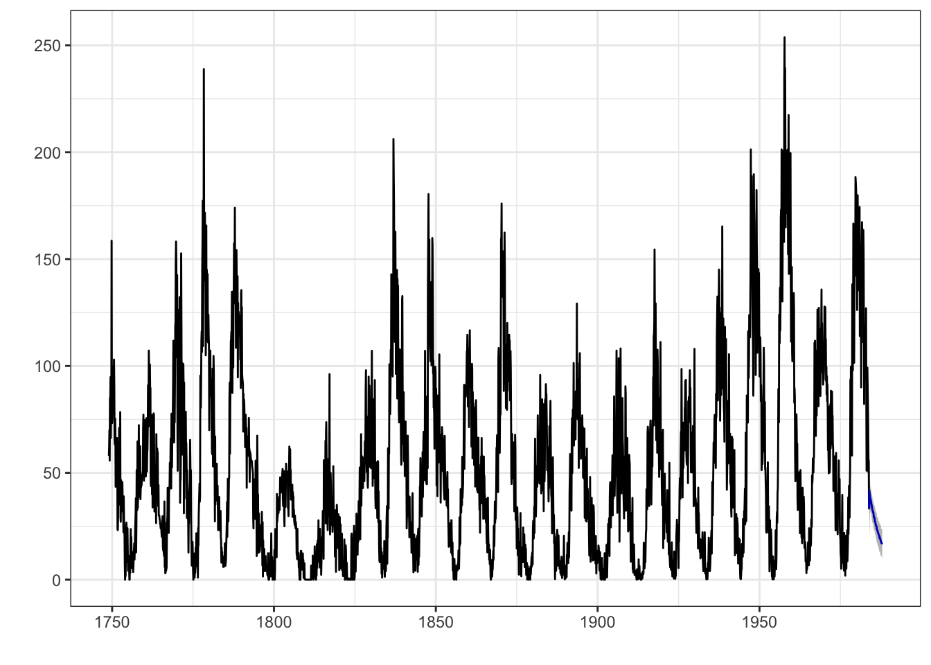
## Elapsed time : 0.167192

# previsão com o modelo
fcast <- ugarchforecast(fit_garch)
# plot(fcast, ask = FALSE)
# desfazendo a diferença
# fcast2 <- fcast
# fcast2@model$modeldata$data <- as.matrix(diffinv(fcast2@model$modeldata$data, xi = y[1]))
# fcast2@model$modeldata$data <- y[-1]
# fcast2@forecast$seriesFor <- as.matrix(diffinv(fcast2@forecast$seriesFor)[-1])
# plot(fcast2)

Exercício 11.33 Veja

1. https://cran.r-project.org/web/packages/rugarch/vignettes/Introduction_to_the_rugarch_package.pdf
2. https://medium.com/analytics-vidhya/arima-garch-forecasting-with-python-7a3f797de3ff

References

Ardia, David, and Lennart F Hoogerheide. 2010. “Bayesian Estimation of the Garch (1, 1) Model with Student-t Innovations.” The R Journal 2 (2): 41–47. https://journal.r-project.org/archive/2010/RJ-2010-014/RJ-2010-014.pdf.

Bollerslev, Tim. 1986. “Generalized Autoregressive Conditional Heteroskedasticity.” Journal of Econometrics 31 (3): 307–27. https://citeseerx.ist.psu.edu/document?repid=rep1&type=pdf&doi=7da8bfa5295375c1141d797e80065a599153c19d.

Bollerslev, Tim, Robert F Engle, and Jeffrey M Wooldridge. 1988. “A Capital Asset Pricing Model with Time-Varying Covariances.” Journal of Political Economy 96 (1): 116–31. https://www.jstor.org/stable/1830713.

Box, George E. P., Gwilym M. Jenkins, and Gregory C. Reinsel. 2008. Time Series Analysis: Forecasting and Control. 4th ed. John Wiley & Sons.

Engle, Robert. 2002. “Dynamic Conditional Correlation: A Simple Class of Multivariate Generalized Autoregressive Conditional Heteroskedasticity Models.” Journal of Business & Economic Statistics 20 (3): 339–50. https://www.tandfonline.com/doi/pdf/10.1198/073500102288618487.

Engle, Robert F. 1982. “Autoregressive Conditional Heteroscedasticity with Estimates of the Variance of United Kingdom Inflation.” Econometrica: Journal of the Econometric Society, 987–1007. http://www.econ.uiuc.edu/~econ508/Papers/engle82.pdf.

Engle, Robert F, and Tim Bollerslev. 1986. “Modelling the Persistence of Conditional Variances.” Econometric Reviews 5 (1): 1–50. https://doi.org/10.1080/07474938608800095.

Engle Robert, F, and Sheppard Kevin. 2001. Theoretical and Empirical Properties of Dynamic Conditional Correlation Multivariate GARCH. UCSD Working Paper NO. https://www.nber.org/system/files/working_papers/w8554/w8554.pdf.

Fonseca, T. C. O., V. S. Cerqueira, H. S. Migon, and C. A. C. Torres. 2019. The Effects of Degrees of Freedom Estimation in the Asymmetric GARCH Model with Student-t Innovations. https://arxiv.org/abs/1910.01398.

Francq, Christian, and Jean-Michel Zakoian. 2010. GARCH Models: Structure, Statistical Inference and Financial Applications. John Wiley & Sons.

Galanos, Alexios. 2025. Rugarch: Univariate GARCH Models. https://cran.r-project.org/package=rugarch.

Matamoros, Izhar Asael Alonzo, and Cristian Andres Cruz Torres. 2020. varstan: An r Package for Bayesian Analysis of Structured Time Series Models with Stan. https://arxiv.org/abs/2005.10361.

Nelson, Daniel B. 1991. “Conditional Heteroskedasticity in Asset Returns: A New Approach.” Econometrica: Journal of the Econometric Society, 347–70. https://www.jstor.org/stable/pdf/2938260.pdf.

Shephard, Neil. 1996. “Statistical Aspects of ARCH and Stochastic Volatility.” In Time Series Models: In Econometrics, Finance and Other Fields. Springer-Science+Business Media, B.V. https://citeseerx.ist.psu.edu/document?repid=rep1&type=pdf&doi=59c8b90f39410447614bcebbfedd985c4bcc59b2.

Trapletti, Adrian, and Kurt Hornik. 2024. Tseries: Time Series Analysis and Computational Finance. https://CRAN.R-project.org/package=tseries.

Vrontos, Ioannis D, Petros Dellaportas, and Dimitris N Politis. 2000. “Full Bayesian Inference for GARCH and EGARCH Models.” Journal of Business & Economic Statistics 18 (2): 187–98. https://www.tandfonline.com/doi/pdf/10.1080/07350015.2000.10524861?casa_token=gESFQI83c2sAAAAA:s-MSp0-EZZzxt_nhFIMZe4rmzCbjRuf380wfFAdo9Gt-XpmLhjNQGJbtkH3Ph9CuMS4BkJOmVqZTFg.

---

22. https://filipezabala.com/data/tsdl/tsdl_20.csv↩︎