11.15 Vetor autorregressivo (VAR)
A abordagem será baseada na biblioteca MTS (Tsay et al. 2022) e em (Tsay 2014).
Exercício 11.40 Veja
11.15.1 Covariância e correlação cruzadas
De acordo com (Diggle 1990, 202–3), a função de covariância cruzada de um processo aleatório estacionário bivariado \(\{(X_t,Y_t)\}\) é o conjunto de números \(\gamma_{xy}(k)\) definido, para cada inteiro \(k\), por \[\begin{equation} \gamma_{xy}(k) = cov(X_{t},Y_{t-k}) \tag{11.57} \end{equation}\]
Note que \(\gamma_{xx}(k)\) e \(\gamma_{yy}(k)\) são as funções de autocovariância de \(\{X_t\}\) e \(\{Y_t\}\) respectivamente, conforme Eq. (11.7). Da mesma forma, \[\gamma_{xy}(-k) = cov(X_t,Y_{t+k}) \\ \hspace{34pt} = cov(Y_{t+k},X_t) \\ \hspace{74pt} = cov(Y_t,X_{t-k}) = \gamma_{yx}(k)\]
A função de correlação cruzada de \(\{(X_t,Y_t)\}\) é \[\begin{equation} \rho_{xy}(k) = \frac{\gamma_{xy}(k)}{\sqrt{\gamma_{xx}(0) \gamma_{yy}(0)}} \tag{11.58} \end{equation}\]
O estimador da função de correlação cruzada é o correlograma cruzado tal que \[\begin{equation} \hat{\rho}_{xy}(k) = \frac{\hat{\gamma}_{xy}(k)}{\sqrt{\hat{\gamma}_{xx}(0) \hat{\gamma}_{yy}(0)}} \tag{11.59} \end{equation}\] onde \[\hat{\gamma}_{xx}(0) = \frac{1}{n} \sum_{t=1}^{n} (x_t-\bar{x})^2, \;\;\;\;\; \hat{\gamma}_{yy}(0) = \frac{1}{n} \sum_{t=1}^{n} (y_t-\bar{y})^2,\] \[\bar{x} = \frac{1}{n} \sum_{t=1}^{n} x_t, \;\;\;\;\; \bar{y} = \frac{1}{n} \sum_{t=1}^{n} y_t,\] \[\hat{\gamma}_{xy}(k) = \left\{ \begin{array}{l l} n^{-1} \sum_{t=k+1}^{n} (x_{t}-\bar{x}) (x_{t-k}-\bar{y}), & \quad k \ge 0\\ n^{-1} \sum_{t=1}^{n+k} (x_{t}-\bar{x}) (x_{t-k}-\bar{y}), & \quad k < 0\\ \end{array} \right. \]
A função stats::ccf calcula as estimativas da correlação cruzada e da covariância cruzada de duas séries univariadas.
Exemplo 11.67 Considere duas séries temporais simladas de ruído branco gaussiano.
set.seed(42)
zt <- matrix(rnorm(200), ncol = 2)
colnames(zt) <- c('z1','z2')
# covariância cruzada
stats::ccf(zt[,'z1'], zt[,'z2'], type = 'covariance',
           ylab = 'cross-covariance', main = 'stats::ccf(type = "covariance")')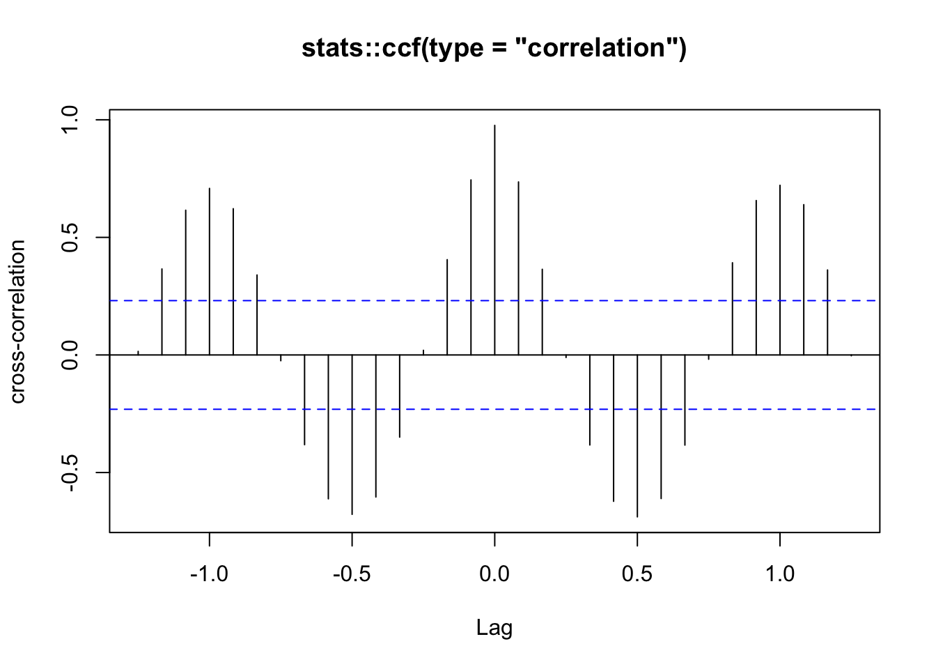
# correlação cruzada
stats::ccf(zt[,'z1'], zt[,'z2'],
           ylab = 'cross-correlation', main = 'stats::ccf(type = "correlation")')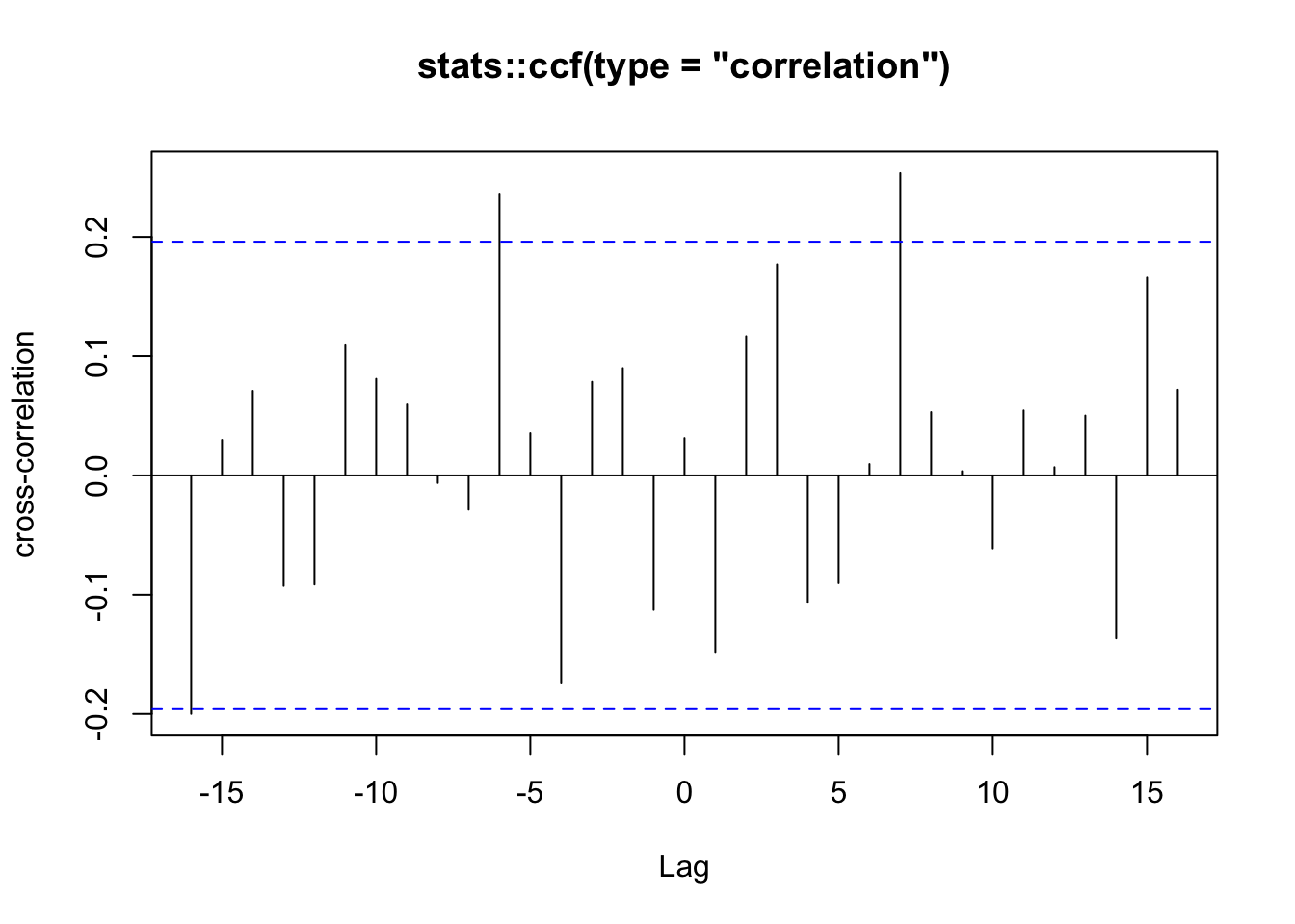
Exemplo 11.68 Considere as séries temporais que das mortes mensais por bronquite, enfisema e asma no Reino Unido entre 1974–1979, ambos os sexos (ldeaths), homens (mdeaths) e mulheres (fdeaths), apresentada por (Diggle 1990, 238).
# correlação cruzada
stats::ccf(mdeaths, fdeaths,
           ylab = 'cross-correlation', main = 'stats::ccf(type = "correlation")')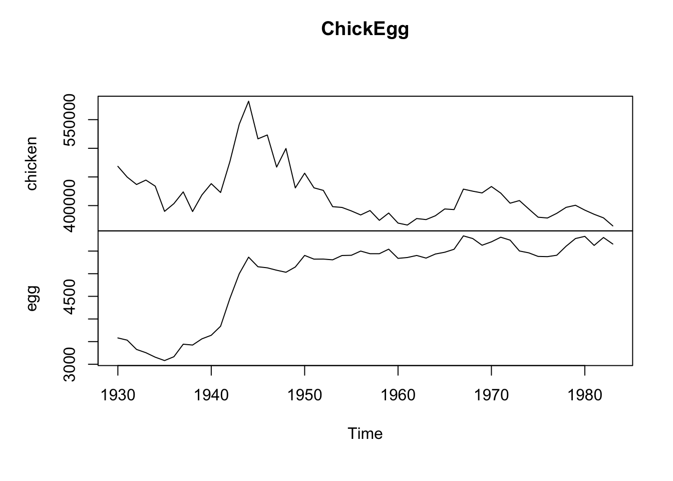
11.15.2 Teste de causalidade de Granger
[U]nder Granger’s framework, we say that \(z_{1t}\) causes \(z_{2t}\) if the past information of \(z_{1t}\) improves the forecast of \(z_{2t}\). (Tsay 2014, 29)
(Granger 1969) propõe o teste de causalidade de Granger, que na verdade testa se uma série \(z_{1t}\) é capaz de prever uma série \(z_{2t}\).
Exemplo 11.69 Baseado na documentação de MTS::GrangerTest().
library(MTS)
set.seed(42)
zt <- matrix(rnorm(200), ncol = 2)
colnames(zt) <- c('z1','z2')
# teste de Granger
MTS::GrangerTest(zt, p = 1)
## Number of targeted zero parameters: 1
## Chi-square test for Granger Causality and p-value: 2.251435 0.1334906
## Constant term:
## Estimates: 0.01752419 -0.1075215
## Std.Error: 0.1047053 0.0906709
## AR coefficient matrix
## AR( 1 )-matrix
## [,1] [,2]
## [1,] 0.0560 0.000
## [2,] -0.0955 -0.106
## standard error
## [,1] [,2]
## [1,] 0.1007 0.0000
## [2,] 0.0868 0.0998
##
## Residuals cov-mtx:
## [,1] [,2]
## [1,] 1.062752024 0.002823729
## [2,] 0.002823729 0.780929140
##
## det(SSE) = 0.8299261
## AIC = -0.1264187
## BIC = -0.04826357
## HQ = -0.0947879## Number of targeted zero parameters: 2
## Chi-square test for Granger Causality and p-value: 3.387032 0.1838719
## Constant term:
## Estimates: 0.02434786 -0.129605
## Std.Error: 0.106115 0.09188827
## AR coefficient matrix
## AR( 1 )-matrix
## [,1] [,2]
## [1,] 0.065 0.000
## [2,] -0.123 -0.124
## standard error
## [,1] [,2]
## [1,] 0.1026 0.000
## [2,] 0.0887 0.102
## AR( 2 )-matrix
## [,1] [,2]
## [1,] -0.00821 0.0000
## [2,] 0.07395 -0.0396
## standard error
## [,1] [,2]
## [1,] 0.1017 0.000
## [2,] 0.0873 0.104
##
## Residuals cov-mtx:
## [,1] [,2]
## [1,] 1.0689678 0.0156749
## [2,] 0.0156749 0.7606777
##
## det(SSE) = 0.8128942
## AIC = -0.08715432
## BIC = 0.06915589
## HQ = -0.02389276## Number of targeted zero parameters: 3
## Chi-square test for Granger Causality and p-value: 7.073532 0.06959063
## Constant term:
## Estimates: 0.01888439 -0.1239715
## Std.Error: 0.1077134 0.09462076
## AR coefficient matrix
## AR( 1 )-matrix
## [,1] [,2]
## [1,] 0.0675 0.000
## [2,] -0.1233 -0.116
## standard error
## [,1] [,2]
## [1,] 0.1037 0.000
## [2,] 0.0899 0.105
## AR( 2 )-matrix
## [,1] [,2]
## [1,] -0.0155 0.0000
## [2,] 0.0772 -0.0198
## standard error
## [,1] [,2]
## [1,] 0.1037 0.000
## [2,] 0.0907 0.107
## AR( 3 )-matrix
## [,1] [,2]
## [1,] 0.0370 0.0000
## [2,] 0.0753 -0.0299
## standard error
## [,1] [,2]
## [1,] 0.104 0.000
## [2,] 0.089 0.106
##
## Residuals cov-mtx:
## [,1] [,2]
## [1,] 1.07692343 0.01998993
## [2,] 0.01998993 0.75362985
##
## det(SSE) = 0.811202
## AIC = -0.02923812
## BIC = 0.2052272
## HQ = 0.06565421Exemplo 11.70 (Thurman et al. 1988) examinam séries temporais anuais dos EUA de 1930 a 1983 sobre produção de ovos e população de galinhas. O objetivo é responder à célebre pergunta: quem veio primeiro, o ovo ou a galinha? (Zeileis and Hothorn 2002) apresentam a série temporal ChickEgg, contendo o conjunto de dados fornecido por Walter Thurman e disponibilizado para R por Roger Koenker, sendo os dados ligeiramente diferentes daqueles analisados em (Thurman et al. 1988). As colunas são
chicken: número de galinhas (população de 1º de dezembro de todas as galinhas dos EUA, excluindo frangos de corte comerciais)egg: número de ovos (produção de ovos nos EUA em milhões de dúzias)
# galinhas granger-causam ovos?
ec1 <- grangertest(egg ~ chicken, order = 1, data = ChickEgg)
ec2 <- grangertest(egg ~ chicken, order = 2, data = ChickEgg)
ec3 <- grangertest(egg ~ chicken, order = 3, data = ChickEgg)
ec4 <- grangertest(egg ~ chicken, order = 4, data = ChickEgg)
ec5 <- grangertest(egg ~ chicken, order = 5, data = ChickEgg)
ec6 <- grangertest(egg ~ chicken, order = 6, data = ChickEgg)
ec7 <- grangertest(egg ~ chicken, order = 7, data = ChickEgg)
ec8 <- grangertest(egg ~ chicken, order = 8, data = ChickEgg)
ec9 <- grangertest(egg ~ chicken, order = 9, data = ChickEgg)
ec10 <- grangertest(egg ~ chicken, order = 10, data = ChickEgg)
ec11 <- grangertest(egg ~ chicken, order = 11, data = ChickEgg)
ec12 <- grangertest(egg ~ chicken, order = 12, data = ChickEgg)
# ovos granger-causam galinhas?
ce1 <- grangertest(chicken ~ egg, order = 1, data = ChickEgg)
ce2 <- grangertest(chicken ~ egg, order = 2, data = ChickEgg)
ce3 <- grangertest(chicken ~ egg, order = 3, data = ChickEgg)
ce4 <- grangertest(chicken ~ egg, order = 4, data = ChickEgg)
ce5 <- grangertest(chicken ~ egg, order = 5, data = ChickEgg)
ce6 <- grangertest(chicken ~ egg, order = 6, data = ChickEgg)
ce7 <- grangertest(chicken ~ egg, order = 7, data = ChickEgg)
ce8 <- grangertest(chicken ~ egg, order = 8, data = ChickEgg)
ce9 <- grangertest(chicken ~ egg, order = 9, data = ChickEgg)
ce10 <- grangertest(chicken ~ egg, order = 10, data = ChickEgg)
ce11 <- grangertest(chicken ~ egg, order = 11, data = ChickEgg)
ce12 <- grangertest(chicken ~ egg, order = 12, data = ChickEgg)
A tabela a seguir apresenta os p-values dos testes realizados, que conforme apontado por (Thurman et al. 1988, 237), os testes “indicam uma clara rejeição da hipótese de que os ovos não causam a doença de Granger. Eles não fornecem tal rejeição à hipótese de que as galinhas não causam a doença de Granger. Portanto, concluímos que o ovo veio primeiro”.
| Ordem | Chicken -> Egg |
Egg -> Chicken |
|---|---|---|
| 1 | 0.8292 | 0.2772 |
| 2 | 0.4215 | 6^{-4} |
| 3 | 0.6238 | 0.003 |
| 4 | 0.8125 | 0.0057 |
| 5 | 0.9131 | 0.0019 |
| 6 | 0.8984 | 0.0064 |
| 7 | 0.7467 | 0.0028 |
| 8 | 0.7619 | 0.0028 |
| 9 | 0.82 | 0.0028 |
| 10 | 0.9438 | 0.0028 |
| 11 | 0.9137 | 0.0028 |
| 12 | 0.9107 | 0.0028 |
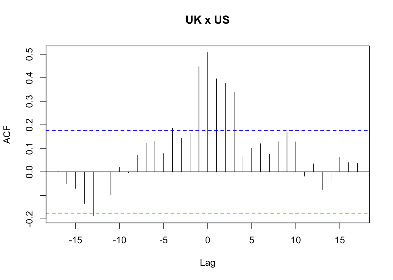
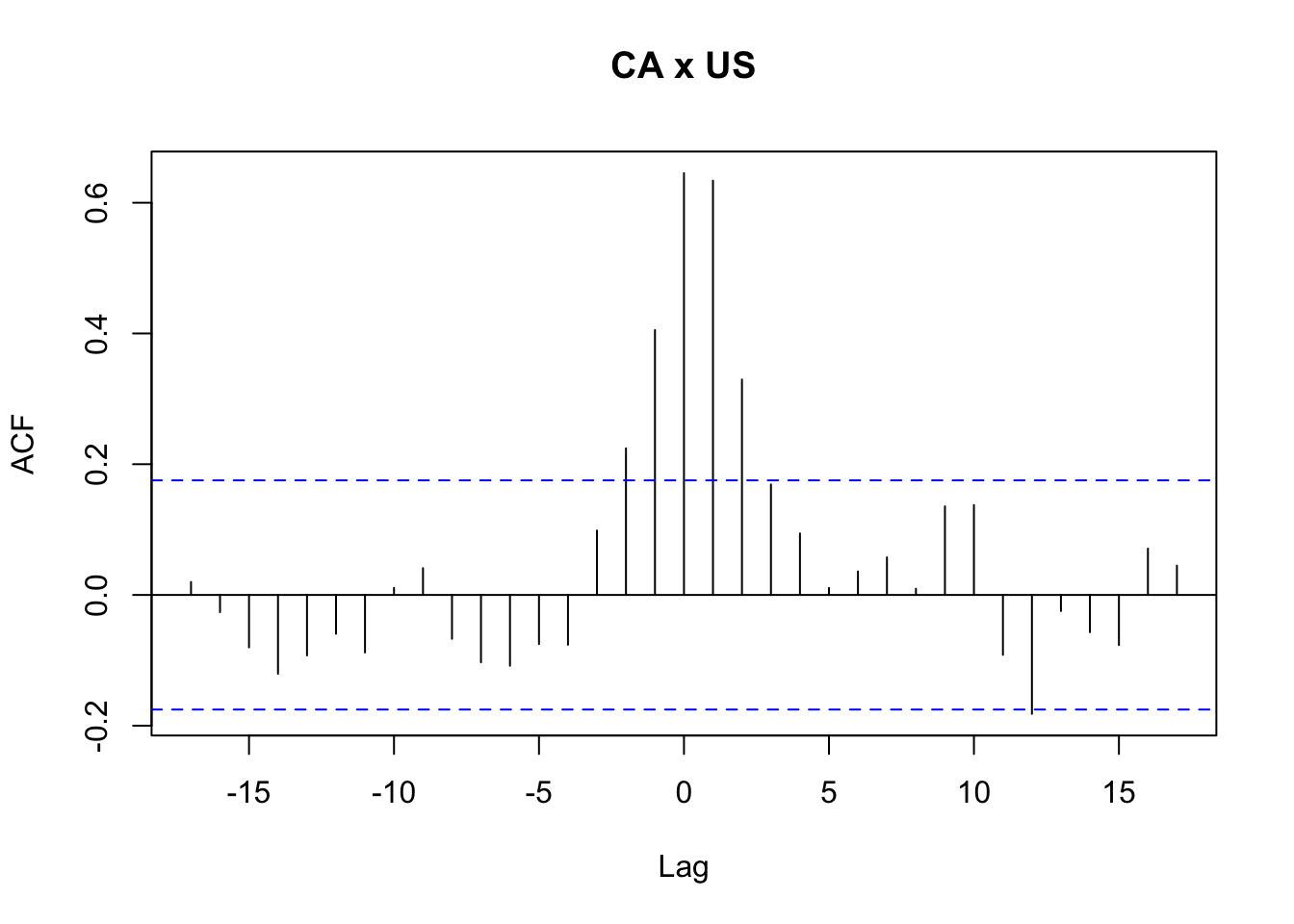
Exemplo 11.71 Baseado nas documentações de MTS::VAR() e MTS::GrangerTest(), baseado no banco de dados qgdp, os produtos internos brutos reais trimestrais do Reino Unido, Canadá e Estados Unidos, do primeiro trimestre de 1980 ao segundo trimestre de 2011.
library(MTS)
data('mts-examples', package = 'MTS')
# Logaritmo natural dos produtos internos brutos
gdp <- log(qgdp[,3:5])
# Diferença multivariada
zt <- MTS::diffM(gdp)
# correlação cruzada
stats::ccf(zt[,'uk'], zt[,'ca'], main = 'UK x CA')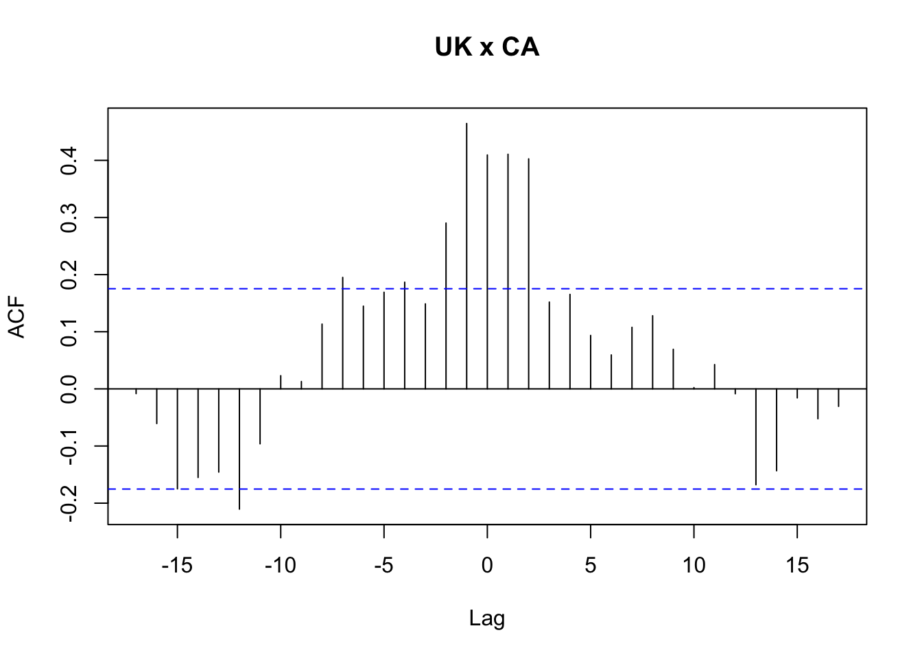
## Number of targeted zero parameters:  2
## Chi-square test for Granger Causality and p-value: 9.393834 0.00912336## Number of targeted zero parameters: 4
## Chi-square test for Granger Causality and p-value: 8.948851 0.06239076
## Constant term:
## Estimates: 0.002104448 0.001231581 0.002895581
## Std.Error: 0.0006685632 0.0007382941 0.000816888
## AR coefficient matrix
## AR( 1 )-matrix
## [,1] [,2] [,3]
## [1,] 0.473 0.000 0.000
## [2,] 0.351 0.338 0.469
## [3,] 0.491 0.240 0.236
## standard error
## [,1] [,2] [,3]
## [1,] 0.0899 0.000 0.0000
## [2,] 0.0949 0.100 0.0926
## [3,] 0.1050 0.111 0.1024
## AR( 2 )-matrix
## [,1] [,2] [,3]
## [1,] 0.151 0.000 0.00000
## [2,] -0.191 -0.175 -0.00868
## [3,] -0.312 -0.131 0.08531
## standard error
## [,1] [,2] [,3]
## [1,] 0.0859 0.0000 0.0000
## [2,] 0.0939 0.0890 0.0953
## [3,] 0.1038 0.0984 0.1055
##
## Residuals cov-mtx:
## [,1] [,2] [,3]
## [1,] 3.042334e-05 2.654091e-06 7.435286e-06
## [2,] 2.654091e-06 2.915817e-05 1.394879e-05
## [3,] 7.435286e-06 1.394879e-05 3.569657e-05
##
## det(SSE) = 2.443371e-14
## AIC = -31.11881
## BIC = -30.80204
## HQ = -30.99013## Number of targeted zero parameters: 6
## Chi-square test for Granger Causality and p-value: 20.55467 0.002204932Exercício 11.41 Google: ‘flowers and bees granger causality’
11.15.3 VAR
Conforme (Tsay 2014, 27), a série temporal multivariada \(\boldsymbol{z}_{t}\) segue um modelo VAR de ordem \(p\), VAR\((p)\), se \[\begin{equation} \boldsymbol{z}_{t} = \boldsymbol{\phi}_0 + \sum_{i=1}^{p} \boldsymbol{\phi}_i \boldsymbol{z}_{t-i} + \boldsymbol{a}_{t} \tag{11.60} \end{equation}\] onde \(\boldsymbol{\phi}_0\) é um vetor constante \(k\)-dimensional e \(\boldsymbol{\phi}_i\) são matrizes \(k \times k\) para \(i>0\), \(\boldsymbol{\phi}_p \ne 0\), e \(\boldsymbol{a}_{t}\) é uma sequência de vetores aleatórios independentes e identicamente distribuídos (iid) com média zero e matriz de covariância positiva-definida \(\Sigma_a\).
Com o operador backshift o modelo pode ser expresso por \[\begin{equation} \boldsymbol{\phi}(B)\boldsymbol{z}_{t} = \boldsymbol{\phi}_0 + \boldsymbol{a}_{t} \tag{11.61} \end{equation}\] onde \[\begin{equation} \boldsymbol{\phi}(B) = \boldsymbol{I}_k - \sum_{i=1}^{p} \boldsymbol{\phi}_i B^i \tag{11.62} \end{equation}\] é uma matriz polinomial de grau \(p\).
11.15.3.1 Estacionariedade
- VAR(1): autovalores absolutos de \(\phi(B)\) menores que 1 garantem modelo VAR(1) estacionário (Tsay 2014, 31)
- VAR(2): a condição necessária e suficiente para a estacionariedade de \(\boldsymbol{Z}_t\) é que todas as soluções da equação determinante \(|\phi(B)| = 0\) são maiores que 1 em valor absoluto. (Tsay 2014, 38)
- VAR\((p)\): a condição necessária e suficiente para a estacionariedade fraca da série VAR\((p)\) é que todas as soluções da equação determinante \(|\phi(B)| = 0\) devem ser maiores que 1 em módulo. (Tsay 2014, 42)
Exemplo 11.72 VAR(1), baseado nas documentações de MTS::VAR() e MTS::VARpred(). Veja Exemplo (exm:grangertest-qgdp).
library(MTS)
data('mts-examples', package = 'MTS')
# Logaritmo natural dos produtos internos brutos
gdp <- log(qgdp[,3:5])
# Diferença multivariada
zt <- MTS::diffM(gdp)
# VAR(1)
m1 <- MTS::VAR(zt, p = 1)
## Constant term:
## Estimates: 0.001713324 0.001182869 0.002785892
## Std.Error: 0.0006790162 0.0007193106 0.0007877173
## AR coefficient matrix
## AR( 1 )-matrix
## [,1] [,2] [,3]
## [1,] 0.434 0.189 0.0373
## [2,] 0.185 0.245 0.3917
## [3,] 0.322 0.182 0.1674
## standard error
## [,1] [,2] [,3]
## [1,] 0.0811 0.0827 0.0872
## [2,] 0.0859 0.0877 0.0923
## [3,] 0.0940 0.0960 0.1011
##
## Residuals cov-mtx:
## [,1] [,2] [,3]
## [1,] 2.893347e-05 1.965508e-06 6.619853e-06
## [2,] 1.965508e-06 3.246932e-05 1.686272e-05
## [3,] 6.619853e-06 1.686272e-05 3.893867e-05
##
## det(SSE) = 2.721916e-14
## AIC = -31.09086
## BIC = -30.88722
## HQ = -31.00813# VAR(1) estacionário pois os autovalores absolutos de $\phi(B)$ são menores que 1
eigen(m1$Phi)$values## [1] 0.70910488 0.08735388 0.05004080## orig 125
## Forecasts at origin: 125
## uk ca us
## [1,] 0.002301 0.002467 0.003630
## [2,] 0.003314 0.003634 0.004582
## [3,] 0.004010 0.004480 0.005280
## [4,] 0.004498 0.005089 0.005774
## Standard Errors of predictions:
## [,1] [,2] [,3]
## [1,] 0.005379 0.005698 0.006240
## [2,] 0.006031 0.006764 0.006787
## [3,] 0.006309 0.007159 0.007043
## [4,] 0.006444 0.007346 0.007168
## Root mean square errors of predictions:
## [,1] [,2] [,3]
## [1,] 0.005464 0.005789 0.006339
## [2,] 0.040704 0.054184 0.039966
## [3,] 0.028021 0.035325 0.028630
## [4,] 0.020427 0.025433 0.020945Exemplo 11.73 VAR(2), veja Exemplo (exm:var1-pred).
# # VAR(2)
# m2 <- MTS::VAR(zt, p = 2)
#
# # Verificar estacionariedade usando o método de Tsay
# # Obter as matrizes de coeficientes
# phi1 <- m2$Phi[,1]  # Matriz \phi_1
# phi2 <- m2$Phi[,2]  # Matriz \phi_2
#
# # Crie a matriz de formulário complementar para VAR(2)
# k <- ncol(zt)  # número de variáveis
# F_matrix <- rbind(
#   cbind(phi1, phi2),
#   cbind(diag(k), matrix(0, k, k))
# )
#
# # Calcule os autovalores da matriz F_matrix
# eigen_vals <- eigen(F_matrix, only.values = TRUE)$values
#
# # Check stationarity condition: all eigenvalues should have modulus < 1
# # (Note: Tsay says roots of |Φ(B)|=0 should be >1, which is equivalent to
# # eigenvalues of companion matrix having modulus < 1)
# is_stationary <- all(Mod(eigen_vals) < 1)
#
# # Print results
# cat("Eigenvalues of companion matrix:\n")
# print(Mod(eigen_vals))
# cat("\nIs the VAR(2) model stationary?", is_stationary, "\n")
#
# # Alternative: using MTS built-in function
# MTS::VARcheck(m2)
#
# # previsão 4 passos à frente
# MTS::VARpred(m2, 4)
11.15.4 VARMA
Conforme (Tsay 2014, 127), a série temporal multivariada \(\boldsymbol{z}_{t}\) é um vetor autorregressivo de média móveis VARMA\((p,q)\), se \[\begin{equation} \boldsymbol{\phi}(B)\boldsymbol{z}_{t} = \boldsymbol{\phi}_0 + \boldsymbol{\theta}(B) \boldsymbol{a}_{t} \tag{11.63} \end{equation}\] onde \[\begin{equation} \boldsymbol{\theta}(B) = \boldsymbol{I}_k - \sum_{i=1}^{q} \boldsymbol{\theta}_i B^i \tag{11.64} \end{equation}\]
Sobre identificabilidade: veja (Tsay 2014, 127).
If the fitted VARMA model is adequate, the residual series \(\{\hat{a}_t\}\) should behave as a \(k\)-dimensional white noises. Thus, we continue to apply the multivariate Ljung–Box statistics (or Portmanteau statistic) (…) to check the serial and cross-correlations of the residuals. (Tsay 2014, 163)
Exemplo 11.74 Baseado nas documentações de MTS::VARMA() e MTS::VARMApred().
phi <- matrix(c(0.2,-0.6,0.3,1.1),2,2)
theta <- matrix(c(-0.5,0,0,-0.5),2,2)
sigma <- diag(2)
m1 <- VARMAsim(300, arlags = c(1), malags = c(1),
               phi = phi, theta = theta, sigma = sigma)
zt <- m1$series
m2 <- MTS::VARMA(zt, p=1, q=1, include.mean = FALSE)
## Number of parameters: 8
## initial estimates: 0.1619 0.3159 -0.7074 1.1276 0.5111 0.0431 0.2171 0.4939
## Par. lower-bounds: 0.0455 0.2668 -0.8292 1.0763 0.3447 -0.0791 0.0431 0.366
## Par. upper-bounds: 0.2783 0.365 -0.5856 1.1789 0.6775 0.1654 0.3912 0.6219
## Final Estimates: 0.1348409 0.3197087 -0.6750053 1.122453 0.5456 0.04958296 0.1749889 0.4531633
##
## Coefficient(s):
## Estimate Std. Error t value Pr(>|t|)
## [1,] 0.13484 0.07097 1.900 0.0574 .
## [2,] 0.31971 0.03126 10.227 < 2e-16 ***
## [3,] -0.67501 0.07771 -8.686 < 2e-16 ***
## [4,] 1.12245 0.03328 33.724 < 2e-16 ***
## [5,] 0.54560 0.06889 7.920 2.44e-15 ***
## [6,] 0.04958 0.04746 1.045 0.2962
## [7,] 0.17499 0.08016 2.183 0.0290 *
## [8,] 0.45316 0.05248 8.634 < 2e-16 ***
## ---
## Signif. codes: 0 '***' 0.001 '**' 0.01 '*' 0.05 '.' 0.1 ' ' 1
## ---
## Estimates in matrix form:
## AR coefficient matrix
## AR( 1 )-matrix
## [,1] [,2]
## [1,] 0.135 0.32
## [2,] -0.675 1.12
## MA coefficient matrix
## MA( 1 )-matrix
## [,1] [,2]
## [1,] -0.546 -0.0496
## [2,] -0.175 -0.4532
##
## Residuals cov-matrix:
## [,1] [,2]
## [1,] 0.96366827 0.03345517
## [2,] 0.03345517 1.08112632
## ----
## aic= 0.09325368
## bic= 0.1920212## Predictions at origin 300
## [,1] [,2]
## [1,] 0.10283 0.2198
## [2,] 0.08414 0.1773
## [3,] 0.06804 0.1422
## [4,] 0.05465 0.1137
## Standard errors of predictions
## [,1] [,2]
## [1,] 0.9817 1.040
## [2,] 1.2546 1.988
## [3,] 1.3811 2.711
## [4,] 1.5306 3.21511.15.5 VARX
The first approach to include exogenous variables in multivariate time series modeling is to use the vector autoregressive model with exogenous variables. In the literature, this type of models is referred to as the VARX models with X signifying exogenous variables. (Tsay 2014, 346)
Seguindo (Tsay 2014, 346), a forma geral do modelo VARX é \[\begin{equation} \boldsymbol{z}_t = \boldsymbol{\phi}_0 + \sum_{i=1}^{p} \boldsymbol{\phi}_i \boldsymbol{z}_{t-i} + \sum_{j=1}^{s} \boldsymbol{\beta}_j \boldsymbol{x}_{t-j} + \boldsymbol{a}_t \tag{11.65} \end{equation}\]
Exemplo 11.75 Baseado no Exemplo 6.2 de (Tsay 2014, 346–50).